HDL - Introduction to Multi GPU Programming

Filled notebook:

Tutorial script files:

Recordings:

Authors: Samuele Papa

Introduction

Using multiple GPUs is a central part in scaling models to large datasets and obtain state of the art performance.

We have seen that, to control multiple GPUs, we need to understand the concepts of distributed computing. The core problem in distributed computing is the communication between nodes, which requires synchronization. Luckily, we are equipped with very limited communication tools, that minimize the chance that problems arise (the specifics are outside the scope of this course, to get more insight into the possible issues, look into concurrent programming, race conditions, deadlocks, resource starvation, semaphores and barriers, and the book Operating Systems Internals and Design Principles).

Tutorial content. To better understand the primitives of communication in a distributed environment, we will begin by looking at some very basic exercises where simple operations are performed. Then, we will look at a more realistic scenario, the computation of the loss in a one-layer classifier (more realistic, but still very simple). Finally, we will learn how to run full-scale training on multiple GPUs and multiple nodes using PyTorch Lightning.

Running the code

The code in these cells is not meant to be run with this notebook. Instead, the files provided should be used in an environment where multiple GPUs are available. This step is not required (all the outputs and explanation of the code are available here), but highly encouraged, as getting familiar with these concepts, especially the more simple primitives, will help when more cryptic errors start appearing in big projects.

Running the scripts can be done, for example, on the GPU partition of the LISA cluster (General Knowledge on how to use the cluster). After getting access using ssh (use WSL on Windows), we can setup the conda environment, by using the module package to load the correct anaconda version and then creating the environment based on the environment.yml file.

To upload the code, the rsync command can be used (on single files, it is possible to do it on folders by adding the -r option):

rsync file account@lisa-gpu.surfsara.nl:~/file

Then, the Anaconda module can be loaded and the environment created using:

module load 2021
module load Anaconda3/2021.05
conda env create -f environment.yml

It will take some time to download the necessary packages.

The main code to run is the following:

srun  -p gpu_shared -n 1 --ntasks-per-node 1 --gpus 2 --cpus-per-task 2 -t 1:00:00 --pty /bin/bash

where with -p gpu_shared we ask for the shared partition where there are GPUs available (other gpu partitions available are listed here), then, we specify that we will be running only 1 task in this node, we want 2 GPUs and we use 2 CPUs as well, for 1 hour. The run consists of executing the command /bin/bash which starts a bash console on the node that we have been assigned. This allows for input of the necessary commands.

Once inside, we can activate the correct anaconda environment and start running the scripts. We need to make sure that both GPUs are exposed to the script, with the following syntax:

python my_script.py

For these examples we will make use of the straightforward interface provided by PyTorch, a good summary is available at the documentation page, where all the details of the functions are shown.

Some useful utilities

The following code will help in the running of the experiments, with some plotting functions and setup of the distributed environment.

import torch
import torch.distributed as dist
import matplotlib.pyplot as plt
import numpy as np
from pathlib import Path
from typing import Optional


def rank_print(text: str):
    """
    Prints a statement with an indication of what node rank is sending it
    """
    rank = dist.get_rank()
    # Keep the print statement as a one-liner to guarantee that
    # one single process prints all the lines
    print(f"Rank: {rank}, {text}.")


def disk(
    matrix: torch.Tensor,
    center: tuple[int, int] = (1, 1),
    radius: int = 1,
    value: float = 1.0,
):
    """
    Places a disk with a certain radius and center in a matrix. The value given to the disk must be defined.
    Something like this:
    0 0 0 0 0
    0 0 1 0 0
    0 1 1 1 0
    0 0 1 0 0
    0 0 0 0 0

    Arguments:
     - matrix: the matrix where to place the shape.
     - center: a tuple indicating the center of the disk
     - radius: the radius of the disk in pixels
     - value: the value to write where the disk is placed
    """
    device = matrix.get_device()
    shape = matrix.shape

    # genereate the grid for the support points
    # centered at the position indicated by position
    grid = [slice(-x0, dim - x0) for x0, dim in zip(center, shape)]
    x_coords, y_coords = np.mgrid[grid]
    mask = torch.tensor(
        ((x_coords / radius) ** 2 + (y_coords / radius) ** 2 <= 1), device=device
    )
    matrix = matrix * (~mask) + mask * value

    return matrix, mask


def square(
    matrix: torch.tensor,
    topleft: tuple[int, int] = (0, 0),
    length: int = 1,
    value: float = 1.0,
):
    """
    Places a square starting from the given top-left position and having given side length.
    The value given to the disk must be defined.
    Something like this:
    0 0 0 0 0
    0 1 1 1 0
    0 1 1 1 0
    0 1 1 1 0
    0 0 0 0 0

    Arguments:
     - matrix: the matrix where to place the shape.
     - topleft: a tuple indicating the top-left-most vertex of the square
     - length: the side length of the square
     - value: the value to write where the square is placed
    """
    device = matrix.get_device()
    shape = matrix.shape
    grid = [slice(-x0, dim - x0) for x0, dim in zip(topleft, shape)]
    x_coords, y_coords = np.mgrid[grid]
    mask = torch.tensor(
        (
            (x_coords <= length)
            & (x_coords >= 0)
            & (y_coords >= 0)
            & (y_coords <= length)
        ),
        device=device,
    )
    matrix = matrix * (~mask) + mask * value

    return matrix, mask


def plot_matrix(
    matrix: torch.Tensor,
    rank: int,
    title: str = "Matrix",
    name: str = "image",
    folder: Optional[str] = None,
    storefig: bool = True,
):
    """
    Helper function to plot the images more easily. Can store them or visualize them right away.
    """
    plt.figure()
    plt.title(title)
    plt.imshow(matrix.cpu(), cmap="tab20", vmin=0, vmax=19)
    plt.axis("off")
    if folder:
        folder = Path(folder)
        folder.mkdir(exist_ok=True, parents=True)
    else:
        folder = Path(".")

    if storefig:
        plt.savefig(folder / Path(f"rank_{rank}_{name}.png"))
    else:
        plt.show()
    plt.close()

When starting the distributed environment, we need to decide a backend between gloo, nccl and mpi. The support for these libraries needs to be already available. The nccl backend should be already available from a GPU installation of PyTorch (CUDA Toolkit is required). On a Windows environment, only gloo works, but we will be running these scripts on a Unix environment.

The second fundamental aspect is how the information is shared between nodes. The method we choose is through a shared file, that is accessible from all the GPUs. It is important to remember that access to this file should be quick for all nodes, so on LISA we will put it in the scratch folder.

The other two parameters are the rank and world_size. The rank refers to the identifier for the current device, while the world size is the number of devices available for computation.

When setting up the distributed environment, the correct GPU device should be selected. For simplicity, we select the GPU that has ID corresponding to the rank, but this is not necessary.

Computation nodes could reside in different nodes, when this happens, using a shared fil

def setup_distrib(
    rank: int,
    world_size: int,
    init_method: str = "file:///scratch/sharedfile",
    backend: str = "nccl",
):
    # select the correct device for this process
    torch.cuda.set_device(rank)

    # initialize the processing group
    torch.distributed.init_process_group(
        backend=backend, world_size=world_size, init_method=init_method, rank=rank
    )

    # return the current device
    return torch.device(f"cuda:{rank}")

Training a model on multiple GPUs is a clear example that we will keep in mind throughout this tutorial to contextualize how to make use of the available primitives of communication in distributed computing.

Initially, we want to give the current weights of the model to every GPU that we are using. To do so, we will broadcast the necessary tensors.

Then, each GPU will collect a subset of the full batch, lets say only 64 out of 256 samples, from memory and perform a forward pass of the model. At the end, we need to compute the loss over the entire batch of 256 samples, but no GPU can fit all of these. Here, the reduction primitive comes to the resque. The tensors that reside in different GPUs are collected and an operation is performed that will reduce the tensors to a single one. This allows for the result of the operation to still fit in memory. We may want to keep thisresult in a single GPU (using reduce) or send it to all of them (using all_reduce).

The operations that we can perform are determined by the backend that we are currently using. When using nccl, the list of available operations is the following: - SUM - AVG (only version 2.10 or higher) - PRODUCT - MIN - MAX

Communication Primitives

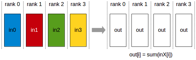
All Reduce

As we can see from the illustration, the all reduce primitive performs an operation between the tensors present in each GPU and replaces them with the result of the operation. The file to run is all_reduce.py.

from utils import setup_distrib, disk, square, rank_print, plot_matrix
import torch.distributed as dist
import torch.multiprocessing as mp
import torch

# operation performed by the reduce
OPERATION = dist.ReduceOp.MAX


def main_process(rank:int, world_size:int=2):
    device = setup_distrib(rank, world_size)
    rank_print("test")
    image = torch.zeros((11,11), device=device)

    if rank == 0:
        rank_image, rank_mask = disk(image, (3,3), 2, rank+1)
    elif rank == 1:
        rank_image, rank_mask = square(image, (3,3), 2, rank+1)

    plot_matrix(rank_image, rank, title=f"Rank {rank} Before All Reduce", name="before_all_reduce", folder="all_reduce")

    # The main operation
    dist.all_reduce(rank_image, op=OPERATION)
    plot_matrix(rank_image, rank, title=f"Rank {rank} After All Reduce Operation: {OPERATION}", name="after_all_reduce", folder="all_reduce")

if __name__ == '__main__':
    mp.spawn(main_process, nprocs=2, args=())

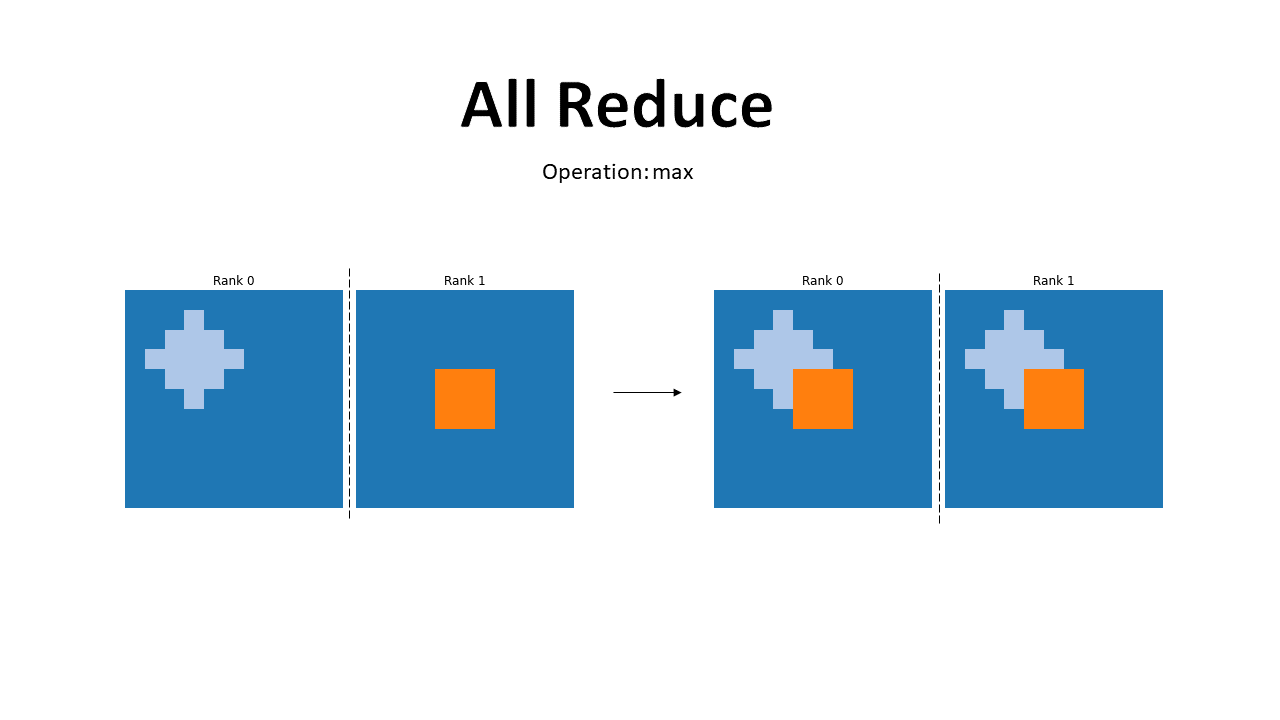
The result of this operation is illustrated in the figure below. The operation is performed between the tensors stored in the different devices and the result is spread across all devices.

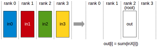
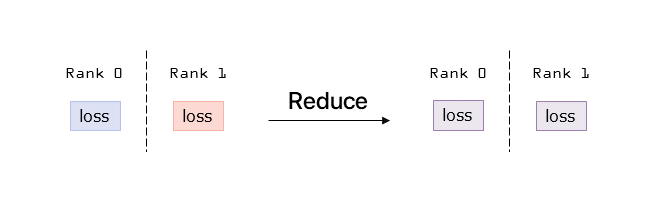
Reduce

As we can see from the illustration, the reduce primitive performs an operation between the tensors present in each GPU and sends the result only to the root rank. In Pytorch, we can define the destination rank. The file to run is reduce.py.

from utils import setup_distrib, disk, square, rank_print, plot_matrix
import torch.distributed as dist
import torch.multiprocessing as mp
import torch
DESTINATION_RANK = 0
OPERATION = dist.ReduceOp.MAX

def main_process(rank, world_size=2):
    device = setup_distrib(rank, world_size)

    image = torch.zeros((11,11), device=device)

    if rank == 0:
        rank_image, rank_mask = disk(image, (4,5), 2, rank+1)
    elif rank == 1:
        rank_image, rank_mask = square(image, (3,3), 2, rank+1)

    plot_matrix(rank_image, rank, title=f"Rank {rank} Before Reduce", name="before_reduce", folder="reduce")

    # The main operation
    dist.reduce(rank_image, dst=DESTINATION_RANK, op=OPERATION)
    plot_matrix(rank_image, rank, title=f"Rank {rank} After Reduce Operation: {OPERATION}", name="after_reduce", folder="reduce")

if __name__ == '__main__':
    mp.spawn(main_process, nprocs=2, args=())

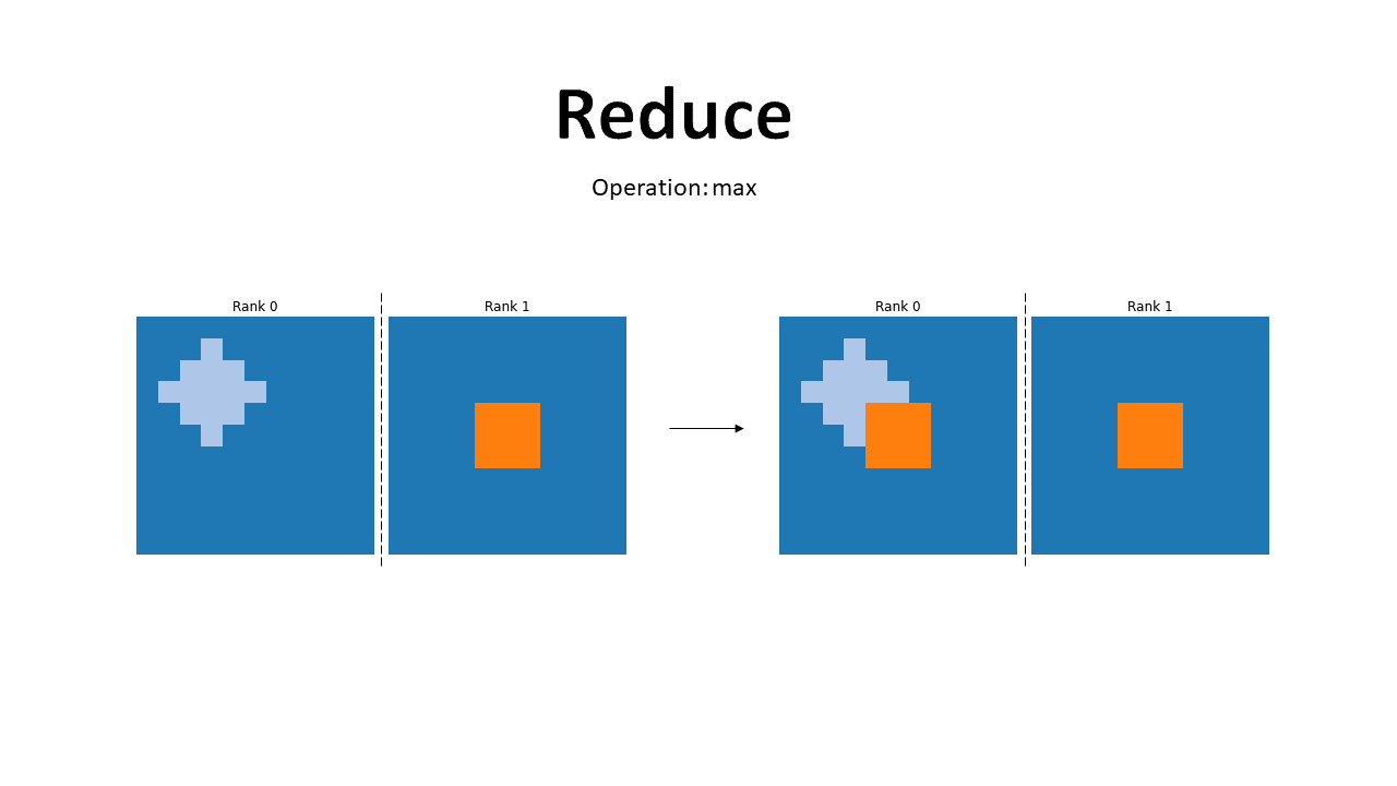
The results are shown below. We can see how only the rank 0, the one we selected, has the result of the operation. This helps in reducing the processing time, if the operation is executed in an asynchronous way, all other GPUs can keep processing while the root one is receiving the result.

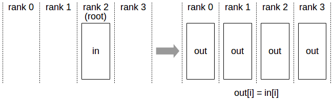
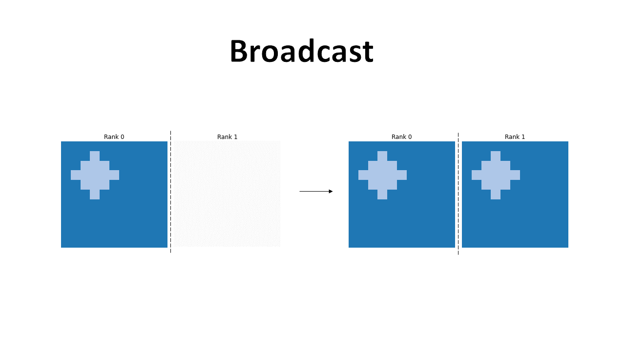
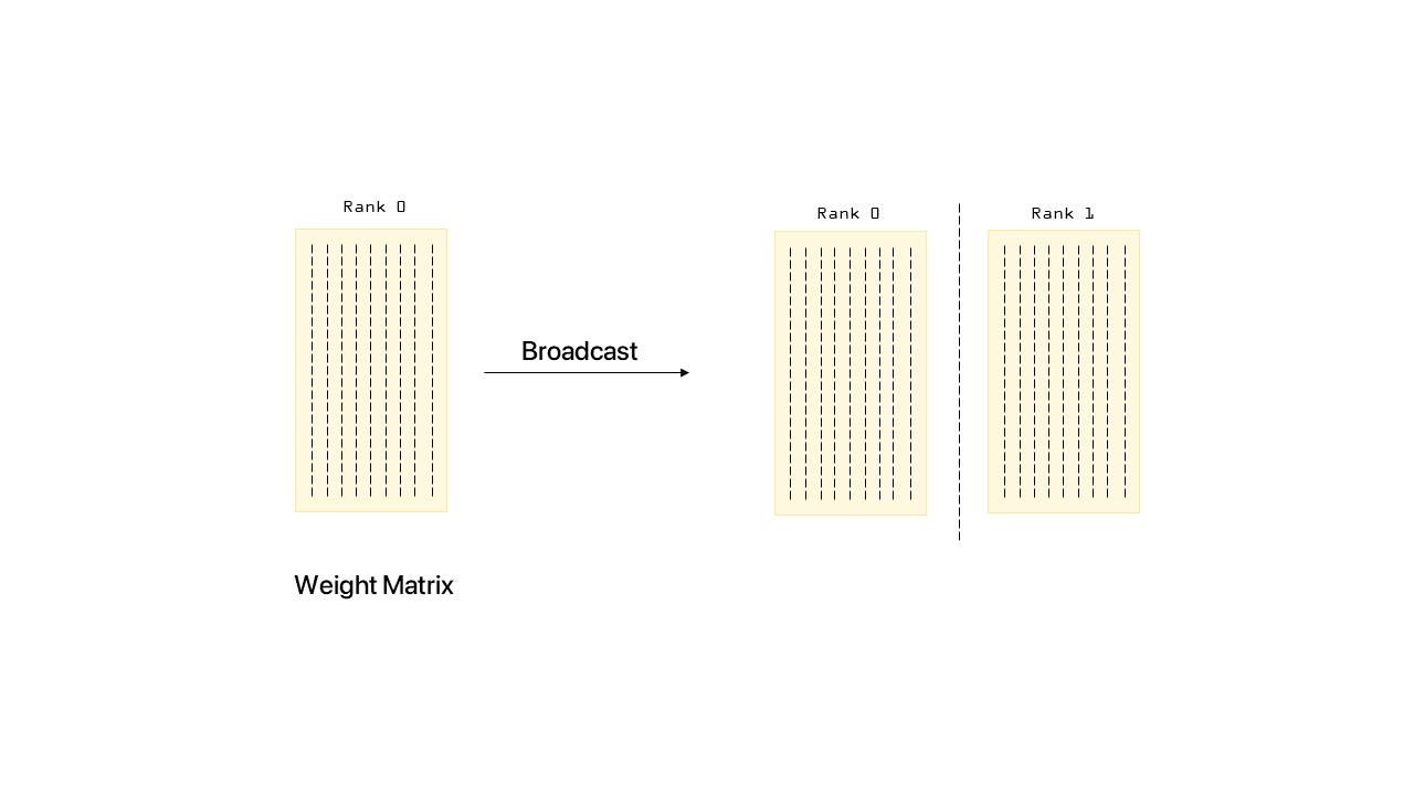
Broadcast

The broadcast operation is fundamental, as it allows to send (broadcast) data from one GPU to all others in the network. The file to run is broadcast.py.

from utils import setup_distrib, disk, square, rank_print, plot_matrix
import torch.distributed as dist
import torch.multiprocessing as mp
import torch
SOURCE_RANK = 0
OPERATION = dist.ReduceOp.MAX

def main_process(rank, world_size=2):
    device = setup_distrib(rank, world_size)

    image = torch.zeros((11,11), device=device)

    if rank == 0:
        rank_image, rank_mask = disk(image, (4,5), 2, rank+1)
    elif rank == 1:
        rank_image, rank_mask = square(image, (3,3), 2, rank+1)

    plot_matrix(rank_image, rank, name="before_broadcast", folder="broadcast")

    # The main operation
    dist.broadcast(rank_image, src=SOURCE_RANK)
    plot_matrix(rank_image, rank, name="after_broadcast", folder="broadcast")


if __name__ == '__main__':
    mp.spawn(main_process, nprocs=2, args=())

In this illustration we see how, the rank 1 GPU gets the correct image after the broadcast is performed.

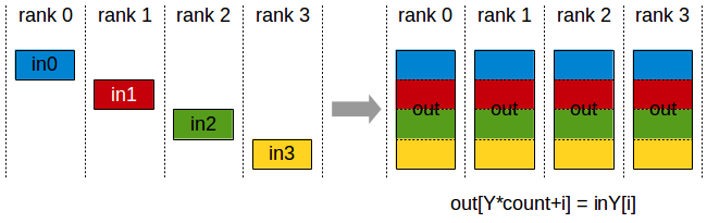
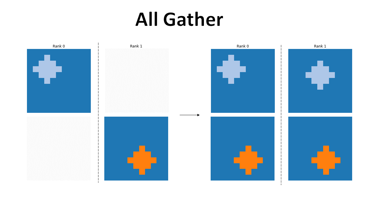
All Gather

The all gather operation allows for all GPUs to have access to all the data processed by the others. This can be especially useful when different operations need to be performed by each GPU, after a common operation has been performed on each subset of the data. It is important to note that the entirety of the data needs to fit in a single GPU, so here the bottleneck won’t be the memory, instead, it will be the processing speed. The file to run is all_gather.py.

from utils import setup_distrib, disk, square, rank_print, plot_matrix
import torch.distributed as dist
import torch.multiprocessing as mp
import torch
def main_process(rank, world_size=2):
    device = setup_distrib(rank, world_size)

    image = torch.zeros((11,11), device=device)

    rank_images = []

    if rank == 0:
        rank_images.append(disk(image, (4,5), 2, rank+1)[0])
    elif rank == 1:
        rank_images.append(disk(image, (7,6), 2, rank+1)[0])

    output_tensors = []
    for _ in range(world_size):
        output_tensors.append(torch.zeros_like(image, device=device))

    plot_matrix(output_tensors[0], rank, title=f"Rank {rank}", name="before_gather_0", folder="all_gather")
    plot_matrix(output_tensors[1], rank, title=f"", name="before_gather_1", folder="all_gather")

    # The main operation
    dist.all_gather(output_tensors, rank_images[0])
    plot_matrix(output_tensors[0], rank, title=f"Rank {rank}", name="after_gather_0", folder="all_gather")
    plot_matrix(output_tensors[1], rank, title=f"", name="after_gather_1", folder="all_gather")


if __name__ == '__main__':
    mp.spawn(main_process, nprocs=2, args=())

Here we can see the result of the all_gather. All GPUs now have access to the data that was initially only present in some of them.

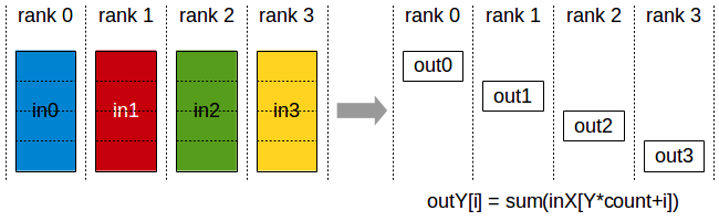
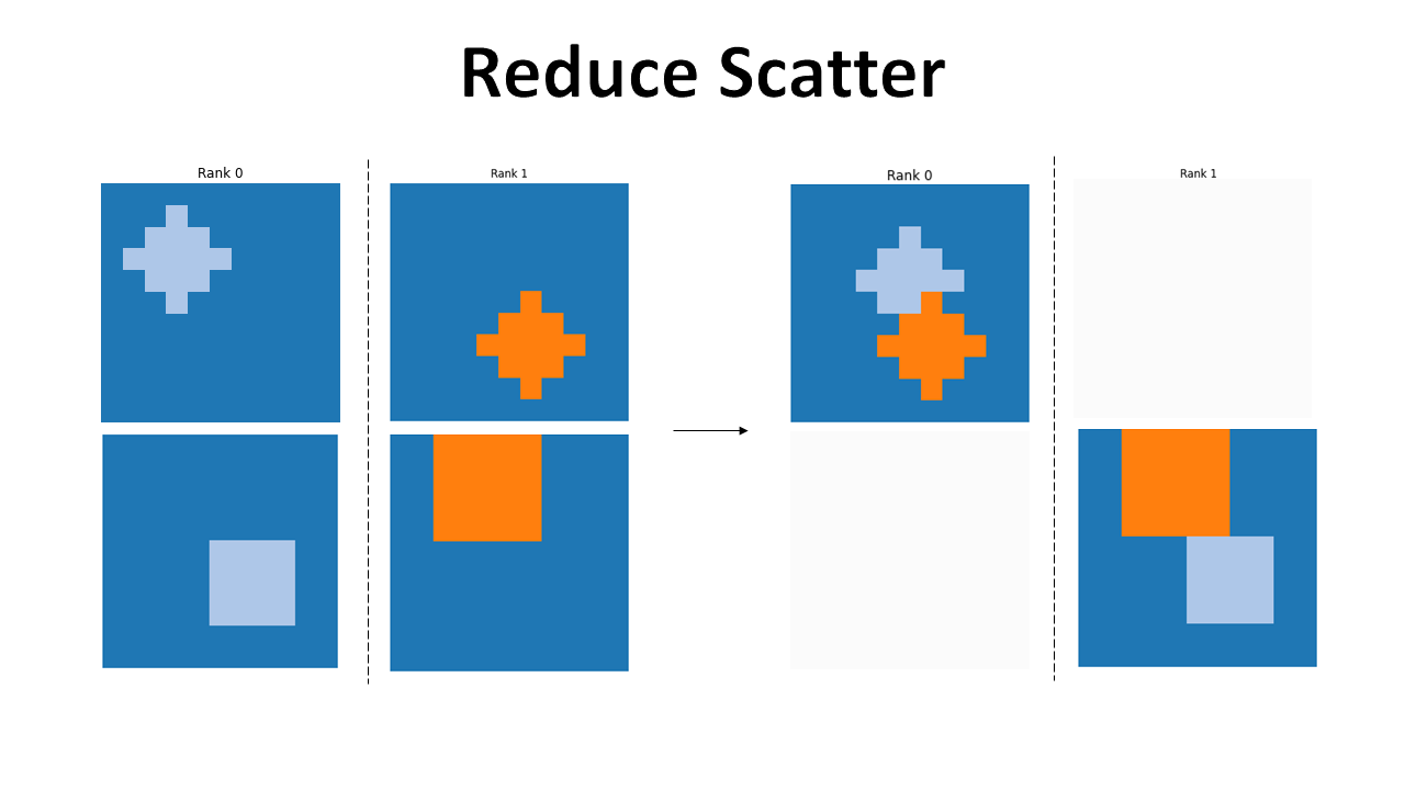
Reduce Scatter

With reduce scatter we can perform an operation on just a subset of the whole data and have each GPU have the partial results. The file to run is reduce_scatter.py.

from utils import setup_distrib, disk, square, rank_print, plot_matrix
import torch.distributed as dist
import torch.multiprocessing as mp
import torch
OPERATION = dist.ReduceOp.MAX
def main_process(rank, world_size=2):
    device = setup_distrib(rank, world_size)

    image = torch.zeros((11,11), device=device)

    input_tensors = []

    if rank == 0:
        input_tensors.append(disk(image, (4,5), 2, rank+1)[0])
        input_tensors.append(square(image, (5,5), 3, rank+1)[0])
    elif rank == 1:
        input_tensors.append(disk(image, (7,6), 2, rank+1)[0])
        input_tensors.append(square(image, (0,2), 4, rank+1)[0])

    output = torch.zeros_like(image, device=device)

    plot_matrix(input_tensors[0], rank, title=f"Rank {rank}", name="before_reduce_scatter_0", folder="reduce_scatter")
    plot_matrix(input_tensors[1], rank, title=f"", name="before_reduce_scatter_1", folder="reduce_scatter")
    plot_matrix(output, rank, title=f"", name="before_reduce_scatter", folder="reduce_scatter")

    # The main operation
    dist.reduce_scatter(output, input_tensors, op=OPERATION)
    plot_matrix(output, rank, title=f"", name="after_reduce_scatter", folder="reduce_scatter")


if __name__ == '__main__':
    mp.spawn(main_process, nprocs=2, args=())

In this figure we see that only one image is available at the end, allowing for the operation to be performed across GPUs while keeping the overall final memory footprint low.

Exercise

An interesting thing to test, if you have access to a multi-GPU environment, is what are the physical limits of the system, and if the processing speed is the same with any number of tensors being loaded into the GPU. Is it more efficient to use a multiple of the number of cores that are processing the data in the GPU, or is the difference in performance negligible? You can investigate these topics through experimentation.

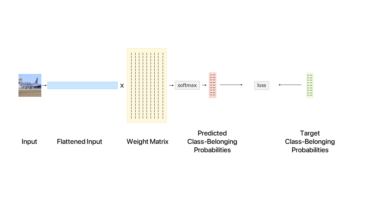
A more comprehensive example

We will now look at a more realistic scenario (code in single_layer.py), the overall process is shown in the figure below.

The first thing we do is to spawn the two processes. In each, we begin by initializing the distributed processing environment.

Then, the datasets needs to be downloaded. Here, I assume that it has not been downloaded yet, and I only let the GPU in rank 0 perform this operation. This avoids having two processes writing in the same file. In order to have the other process wait for the first one to download, a barrier is used. The working principle is very simple, when a barrier is reached in the code, the process waits for all other processes to also reach that point in the code. Here we see how this can be a very useful construct in parallel computing, all processes require the dataset to be downloaded before proceeding, so one of them starts the download, and all wait until it’s done.

Then we initialize the weights, only in the rank 0 GPU, and broadcast them to all other GPUs. This broadcast operation is performed asynchronously, to allow for the rank 0 GPU to start loading images before the rank 1 has received the weights. This operation is akin to what DataParallel does, which is slowing the processing of the other GPUs down, waiting to receive the weights from the root GPU.

Each GPU will then load the images from disk, perform a product to find the activations of the next layer and calculate a softmax to get class-belonging probabilities.

Finally, the loss is computed by summing over the dimensions and a reduction with sum is performed to compute the overall loss over the entire batch.

import torch
import torch.distributed as dist
import torch.multiprocessing as mp
import torchvision
from torchvision import transforms
from utils import rank_print

DSET_FOLDER = "/scratch/"


def main_process(rank, world_size=2):
    print(f"Process for rank: {rank} has been spawned")

    # Setup the distributed processing
    device = setup_distrib(rank, world_size)

    # Load the dataset in all processes download only in the first one
    if rank == 0:
        dset = torchvision.datasets.CIFAR10(DSET_FOLDER, download=True)

    # Make sure download has finished
    dist.barrier()

    # Load the dataset
    dset = torchvision.datasets.CIFAR10(DSET_FOLDER)

    input_size = 3 * 32 * 32  # [channel size, height, width]
    per_gpu_batch_size = 128
    num_classes = 10
    if dist.get_rank() == 0:
        weights = torch.rand((input_size, num_classes), device=device)
    else:
        weights = torch.zeros((input_size, num_classes), device=device)

    # Distribute weights to all GPUs
    handle = dist.broadcast(tensor=weights, src=0, async_op=True)
    rank_print(f"Weights received.")

    # Flattened images
    cur_input = torch.zeros((per_gpu_batch_size, input_size), device=device)

    # One-Hot encoded target
    cur_target = torch.zeros((per_gpu_batch_size, num_classes), device=device)
    for i in range(per_gpu_batch_size):
        rank_print(f"Loading image {i+world_size*rank} into GPU...")
        image, target = dset[i + world_size * rank]
        cur_input[i] = transforms.ToTensor()(image).flatten()
        cur_target[i, target] = 1.0

    # Compute the linear part of the layer
    output = torch.matmul(cur_input, weights)
    rank_print(f"\nComputed output: {output}, Size: {output.size()}.")

    # Define the activation function of the output layer
    logsoftm = torch.nn.LogSoftmax(dim=1)

    # Apply activation function to output layer
    output = logsoftm(output)
    rank_print(f"\nLog-Softmaxed output: {output}, Size: {output.size()}.")

    loss = output.sum(dim=1).mean()
    rank_print(f"Loss: {loss}, Size: {loss.size()}")

    # Here the GPUs need to be synched again
    dist.reduce(tensor=loss, dst=0, op=dist.ReduceOp.SUM)

    rank_print(f"Final Loss: {loss/world_size}")


if __name__ == "__main__":
    mp.spawn(main_process, nprocs=2, args=())

PyTorch Lightning

When you have your Pytorch Lightning module defined, scaling to multiple GPUs and multi nodes is very straightforward (more details here):

trainer = Trainer(gpus=8, strategy="ddp")

Yes, seems impossible, but it’s real. In most cases this is all you need to run multi GPU training.

Conclusion

We have seen how the basic collective primitives for communication work in a multi GPU environment. The reduction and broadcast operations are maybe the most important ones, allowing for delivery of data to all nodes and to perform mathematical operations on the data present in all the nodes.

We have seen how we can use these collectives to perform a calculation of the loss of a neural network, but the same can be extended to any type of parallelizable computation.

Finally, we saw how simple it is to set a PyTorch Lightning training to use multiple GPUs.

References

Pytorch Documentation on Distributed Communication. https://pytorch.org/docs/stable/distributed.html

NVIDIA NCCL Developer Guide. https://docs.nvidia.com/deeplearning/nccl/user-guide/docs/overview.html

PyTorch Lightning Multi-GPU Training. https://pytorch-lightning.readthedocs.io/en/stable/advanced/multi_gpu.html

Concurrent Programming and Operating Systems. Stallings, William. Operating Systems : Internals and Design Principles. Upper Saddle River, N.J. :Prentice Hall, 2001.