Part 3.2: Looping Pipelines

Filled notebook:

Author: Phillip Lippe

In Part 3.1, we have seen how we can use pipeline parallelism to distribute a model across multiple GPUs. A remaining difficulty in pipeline parallelism is the pipeline bubble, which is the time that devices are idle while waiting for the next stage to finish. Micro-batching, as discussed in Part 3.1, improves the efficiency of pipeline parallelism, but some drawbacks still remain. For example, while the pipeline bubble has been reduced, our devices are still idle for model_axis_size - 1 stage executions of a single microbatch. One way of reducing this idle time is by making the microbatches smaller and execute more in sequence, but as discussed before, it becomes difficult to fully utilize the devices with tiny batch sizes. So, can we instead reduce the time of the second factor, i.e. the stage execution? As it turns out, we can, and one option for it are Looping Pipelines introduced by Narayanan et al., 2021, which will be the focus of this notebook.

So far, we have split the model into consecutive stages of layers. For instance, for a model with 8 layers and 4 model devices, we would place the first two layers on the first device, the next two layers on the second device, and so on. However, we can also split the model into non-consecutive stages, and loop over our devices. For instance, we could place the first layer on the first device, the second layer on the second device, and so on, until we place the fifth layer on the first device again. This split of layers is shown in the figure below.

A microbatch is then passed through the looped pipeline in a similar way as before, but the output of the last stage, when it executes layer 4, is passed to the first stage again to continue with layer 5. Now, every stage execution takes only have the time as before, since we are executing half the layers. Furthermore, compared to reducing microbatch size, the stage reduction doesn’t reduce efficiency since the layers would have been executed sequentially anyways.

As long as we have more or an equal number of microbatches as number of model devices, which we anyways need to keep the pipeline efficient, we can keep the devices busy for a large amount of the time. This is because the output of the first stage is passed to the second stage, and so on, until the output of the last stage is passed to the first stage again. This way, the looping does not introduce an additional bubble while reducing the execution of the individual stages. The computation graph for the forward pass will look similar as in the figure below:

Note that if we have more microbatches than model devices, we can either decide to first finish all microbatches of its earlier layer before moving on to the next layer (breadth-first), or start with the next layer as early as possible (depth-first). We will discuss the differences between the two approaches below, but support both in our implementation.

Compared to the estimated execution time of the original pipeline (shown in gray), the execution time of the looping pipeline is significantly reduced, and the devices are kept busy for a larger portion of the time. We have to note though, that this computation graph takes a strong simplification by ignoring the communication costs, which we discuss in more detail in the next section.

In this notebook, we will implement a looping pipeline for a simple model and compare it to the original pipeline. We will also discuss the differences between the depth-first and breadth-first approaches, and how we can implement them.

Prerequisites

Before starting the implementation, we set up the basic environment and utility functions we have seen from previous notebooks. We download the python scripts of the previous notebooks below. This is only needed when running on Google Colab, and local execution will skip this step automatically.

import os
import urllib.request
from urllib.error import HTTPError

# Github URL where python scripts are stored.
base_url = "https://raw.githubusercontent.com/phlippe/uvadlc_notebooks/master/docs/tutorial_notebooks/scaling/JAX/"
# Files to download.
python_files = ["single_gpu.py", "data_parallel.py", "pipeline_parallel.py", "utils.py"]
# For each file, check whether it already exists. If not, try downloading it.
for file_name in python_files:
    if not os.path.isfile(file_name):
        file_url = base_url + file_name
        print(f"Downloading {file_url}...")
        try:
            urllib.request.urlretrieve(file_url, file_name)
        except HTTPError as e:
            print(
                "Something went wrong. Please try to download the file directly from the GitHub repository, or contact the author with the full output including the following error:\n",
                e,
            )

As before, we simulate 8 devices on CPU to demonstrate the parallelism without the need for multiple GPUs or TPUs. If you are running on your local machine and have multiple GPUs available, you can comment out the lines below.

from utils import simulate_CPU_devices

simulate_CPU_devices()

We now import our standard libraries.

import functools
from pprint import pprint
from typing import Any, Callable, Dict, Tuple

import flax.linen as nn
import jax
import jax.numpy as jnp
import numpy as np
import optax
from flax.struct import dataclass
from jax.experimental.shard_map import shard_map
from jax.sharding import Mesh
from jax.sharding import PartitionSpec as P
from ml_collections import ConfigDict

# Helper types
PyTree = Any
Parameter = jax.Array | nn.Partitioned
Metrics = Dict[str, Tuple[jax.Array, ...]]

We also import the utility functions from the previous notebooks. We also import several functions from the previous notebook Part 3.1, since many utilities like the model and the training step can be reused. It is recommended to have a look at the previous notebook to understand the details of the implementation.

from pipeline_parallel import (
    PPClassifier,
    get_default_pp_classifier_config,
    train_pipeline_model,
    train_step_pp,
)
from single_gpu import Batch, TrainState, get_num_params, print_metrics

Looping Pipelines

With all functions set up, we can now start implementing the looping pipeline. We first discuss the communication overlap in the looping pipeline, and then dive deeper into the implementation.

Importance of Communication Overlap

Looping pipelines reduce the pipeline bubble, but for the cost of increased communication overhead. Consider num_loops to be the number of separate layers per stage (a standard pipeline has num_loops=1). For a single microbatch, a standard pipeline requires model_axis_size - 1 communications (i.e. once between each stage pair), while a looping pipeline requires model_axis_size * num_loops - 1 communications (i.e. multiple loops over each stage pair). Many frameworks like JAX support asynchronous communication, which means that the communication can overlap with the computation. However, this is only possible if the computation does not depend on the communicated values. For instance, if the output of stage 1 is communicated to stage 2, stage 2 may not be able to start its computation before the communication is finished (if there are computations that are independent of the input, e.g. RoPE embeddings, they can be executed in parallel). Meanwhile, if stage 1 may not have to wait for stage 4 to finish its computation if it uses the original input and is not yet in the looping regime. Thus, while the looping pipeline seems always superior over the non-looping version in ideal conditions, we may not be able to ignore the communication cost in practice and need to take them into account. An example comparison of GPU utilization between (a) no communication cost versus (b) common communication cost is shown below (figure credit:Joel Lamy-Poirier, 2023). We will have a closer discussion on this in the next notebook on tensor parallelism.

Pipeline parallelism is usually combined with data parallelism to further increase the global batch size. This adds another layer of communication, since after having calculated the gradients for a stage, we need to communicate them across data devices. From our previous discussion, we know that overlapping communication with computation is crucial for efficient distributed training. In standard pipelines, we can only start communicating the gradients after the last microbatch per stage has finished. Depending on the communication cost, this can lead to a significant idle time of the devices, as shown in the computation diagram below (figure credit:Joel Lamy-Poirier, 2023).

In looping pipelines, we can instead structure our layer execution such that we can start communicating gradients earlier. For instance, the breadth-first strategy (Joel Lamy-Poirier, 2023) follows the setup that each stage first finishes all microbatches of its earlier layer before moving on to the next layer. This way, in the backward pass, we finish calculating all gradients for the later layers before having done the computation of the earlier layers. This allows us to start communicating the gradients of the later layers earlier, and overlap it with the computation of the gradients of the early layers. The final communication of the earlier layers will be cheaper than the non-looped version, since significantly fewer gradients need to be communicated (specifically 1/num_loops). The computation diagram for the backward pass of the breadth-first strategy is shown above. An alternative strategy is the depth-first strategy, which starts with the next layer as early as possible, but cannot take advantage of the early communication of the gradients as well as the breadth-first strategy. While we will mainly focus on the breadth-first strategy, our implementation is designed to support both strategies.

Note: in the current implementation version, we may not support asynchronous gradient communication on GPU. This is because the current implementation needs to stack the parameters over the looping axis within the pipeline, in order to support the SPMD jitting of the pipeline. Thus, the gradients are only communicated once the gradients for all parameters in the pipeline have been calculated. To keep the implementation simple, we will neglect the asynchronous gradient communication for now, and focus on the forward pass of the pipeline. A future version of the implementation may support asynchronous gradient communication once we find a simple way for it, and we will update the notebook accordingly.

Looping Pipeline Implementation

Let’s focus now on the implementation of looping pipelines. Compared to the non-looped pipeline, we need to take care of two additional aspects: (1) the looping communication between the last and first stage, and (2) the execution of different layers on a single device over iterations. We will start with the first aspect, and then discuss the second aspect.

If we had the same number of microbatches as model devices, the communication between the last stage and the first stage would not be any different from the communication between any other stage pair after we processed the original input batches. However, if we have more microbatches than model devices, we will need to buffer the outputs of the last stage until we have processed all microbatches of the earlier layers, since the first stage is not ready to process the output of the last stage yet. Thus, at each iteration, we need to check on device 0 which microbatch the communicated features of the last stage belong to and buffer accordingly. We can do this by simply determining the index of the microbatch by using the iteration index, and overwrite the respectively indexed subarray inputs of the first stage with the buffered features. For example, with four devices, the last stage will process the first microbatch at iteration 3 (zero-indexed). At the subsequent communication, we overwrite inputs[0] on device 0 with the communicated features from the last stage. We can then continue with the execution of the first stage as usual and continue iterating over the input array. This results in a computation graph similar to the one shown below (we show processing of 6 instead of 4 microbatches to visualize the buffering mechanism).

The second aspect we need to take care of are the different layers we need to execute at different iterations. Note that these layer indices are not the same across stages: in the diagram above, the first stage will have to switch from layer 0 to layer 4 earlier than the last stage from layer 3 to 7. We can handle this by using the iteration index to determine the layer index we need to execute, and pass the sub-indexed parameters of the respective layer to the stage.

To keep our implementation as general as possible, we will explicitly pass these “switching” indices to the pipeline function. For this, we implement a PipelineState below, which contains: * inputs: The input array, which is the original input array at the first iteration, and is used as buffer for the output of the last stage in subsequent loops. * outputs: The output array, which will store the output of the final layer of the last stage. * input_indices: The indices indicating which microbatch to process at each iteration on the first stage. * output_indices: The indices indicating into which output array to write the output of the last stage at each iteration. If -1, the features will not be stored in the outputs array. * update_indices: The indices indicating which input array index to buffer the last communicated features in. If -1, the features will not be buffered (e.g. initial iterations where the last stage has not received any viable input yet). * params_indices: The index of the layer to execute at each iteration. * last_state: The last communicated features between stages. * rngs: The random number generator keys for the layers (e.g. dropout).

@dataclass
class PipelineState:
    inputs: jax.Array
    outputs: jax.Array
    input_indices: jax.Array
    output_indices: jax.Array
    update_indices: jax.Array
    params_indices: jax.Array
    last_state: jax.Array
    rngs: PyTree

Using this pipeline state, we can implement a single step of the looped pipeline in an SPMD fashion. We first check if we need to buffer the last communicated features, and if so, we do so. We then determine the input to the current stage, which is the last communicated features for all stages except the first. For the first stage, we use the original input array indexed at the current input_indices. We then execute the layer indexed at the current params_indices. For easiest selection of the parameters, we will stack the parameters over the first axis and select them before executing the module.apply_fn. Note that for easiests handling, we use an explicit apply_fn since initializing the right number of parameters within this function is not straightforward. More on it later.

After applying the model, we determine whether the features need to be stored in the outputs array. If so, we do so. Finally, we communicate the last state to the next stage, and return the new pipeline state.

def execute_looping_pipeline_step(
    index: jax.Array | int,
    state: PipelineState,
    *args,
    module: nn.Module,
    params: PyTree,
    model_axis_name: str,
    **kwargs,
) -> PipelineState:
    """Single micro-batch pipeline step with loopback communication.

    Args:
        index: Pipeline step index (between 0 and num_loops * num_microbatches + num_stages - 2).
        state: State of the pipeline, including indices for controlling the execution.
        *args: Additional arguments to the module.
        module: Flax module representing the stage layer to execute.
        params: PyTree of parameters. The params for all layers should be stacked along the first axis.
        model_axis_name: Name of the model axis in the mesh/shard_map.
        **kwargs: Additional keyword arguments to the module.

    Returns:
        New state of the pipeline after the execution of the pipeline step, with potentially updated
        inputs, outputs, rngs, and last_state arrays.
    """
    num_stages = jax.lax.psum(1, model_axis_name)
    input_index = state.input_indices[index]
    output_index = state.output_indices[index]
    update_index = state.update_indices[index]
    params_index = state.params_indices[index]
    # Update inputs with last state. If update_index is -1, do not update.
    # This is used to buffer the communications back to first stage.
    clipped_update_index = jnp.clip(update_index, 0, state.inputs.shape[0] - 1)
    inputs = jax.lax.dynamic_update_index_in_dim(
        state.inputs,
        jnp.where(update_index >= 0, state.last_state, state.inputs[clipped_update_index]),
        clipped_update_index,
        axis=0,
    )
    # Select input of the current stage. For all stages except the first stage,
    # the input is the last output of the previous stage (i.e. last_state).
    step_input = jnp.where(
        input_index >= 0,
        inputs[input_index],
        state.last_state,
    )
    # Apply the module to the input. Select the right set of parameters based
    # on the loop index.
    rngs = jax.tree_map(lambda rng: jax.random.split(rng, 2), state.rngs)
    rngs, step_rngs = jax.tree_map(lambda x: x[0], rngs), jax.tree_map(lambda x: x[1], rngs)
    params = jax.tree_map(lambda x: x[params_index], params)
    output = module.apply(params, step_input, *args, **kwargs, rngs=step_rngs)
    # Update outputs with the output of the current stage. If output_index is -1,
    # do not update. This is used to buffer the final outputs of the last stage.
    clipped_output_index = jnp.clip(output_index, 0, state.outputs.shape[0] - 1)
    outputs = jax.lax.dynamic_update_index_in_dim(
        state.outputs,
        jnp.where(output_index >= 0, output, state.outputs[clipped_output_index]),
        clipped_output_index,
        axis=0,
    )
    # Communicate the last output to the next stage.
    last_state = jax.lax.ppermute(
        output,
        model_axis_name,
        perm=[(i, (i + 1) % num_stages) for i in range(num_stages)],
    )
    return state.replace(
        inputs=inputs,
        outputs=outputs,
        last_state=last_state,
        rngs=rngs,
    )

With the single step set up, we can now write a small helper function to prepare the input_indices, output_indices, update_indices, and params_indices for a respective device. We will use this function to prepare the indices for all devices, and then use them to initialize the pipeline state. The indices follow the breadth-first strategy, as discussed in the previous paragraphs.

def prepare_looping_pipeline_indices(
    num_loops: int, num_microbatches: int, num_stages: int, stage_index: jax.Array | int
) -> Dict[str, jax.Array]:
    """Prepare indices for controlling the execution of the looping pipeline.

    Args:
        num_loops: Number of loops in the pipeline, or separate stage layers per device. num_loops=1 is equivalent to a non-looping pipeline.
        num_microbatches: Number of microbatches to split the batch into.
        num_stages: Number of stages/devices the pipeline is distributed over.
        stage_index: Index of the stage/device in the pipeline.

    Returns:
        Dictionary of indices for controlling the execution of the pipeline.
    """
    num_iterations = num_loops * num_microbatches + num_stages - 1
    index_array = -jnp.ones((num_iterations,), dtype=jnp.int32)
    # Only first stage uses inputs. Looping communications from last
    # stage are buffered in the inputs, so we repeatedly iterate over
    # the inputs.
    input_indices = jnp.where(
        stage_index == 0,
        index_array.at[: num_loops * num_microbatches].set(
            jnp.tile(jnp.arange(num_microbatches), reps=(num_loops,))
        ),
        index_array,
    )
    # For the first stage, identify input indices that we use to buffer
    # the communications from the last stage. For all other stages, we
    # use the last state from the previous stage as input.
    update_indices = jnp.where(
        stage_index == 0,
        index_array.at[num_stages : num_stages + (num_loops - 1) * num_microbatches].set(
            jnp.tile(jnp.arange(num_microbatches), reps=(num_loops - 1,))
        ),
        index_array,
    )
    # For the last stage, we use the outputs of the last loop as the
    # final outputs.
    output_indices = jnp.where(
        stage_index == num_stages - 1,
        index_array.at[-num_microbatches:].set(jnp.arange(num_microbatches)),
        index_array,
    )
    # For all stages, we iterate over the parameters of the different loops.
    # We use the 0-index for indices that fall into the pipeline bubble.
    params_indices = jnp.zeros_like(index_array)
    for i in range(num_loops):
        start_index = stage_index + i * num_microbatches
        params_indices = jax.lax.dynamic_update_slice_in_dim(
            params_indices,
            jnp.full(shape=(num_microbatches,), fill_value=i, dtype=params_indices.dtype),
            start_index,
            axis=0,
        )
    return {
        "input": input_indices,
        "output": output_indices,
        "update": update_indices,
        "params": params_indices,
    }

The easiest way of understanding these indices is to print them for a simple example. Let’s do this for a model with three devices, two loops, and four microbatches. In this setup, we get the following indices for the three devices:

num_stages = 3
num_loops = 2
num_microbatches = 4
for i in range(num_stages):
    indices = prepare_looping_pipeline_indices(
        num_loops=num_loops,
        num_microbatches=num_microbatches,
        num_stages=num_stages,
        stage_index=i,
    )
    s = ["step  : " + " ".join(f"{t:2d}" for t in range(len(indices["input"])))]
    for k, v in indices.items():
        s.append(f"{k:6s}: " + " ".join(f"{t:2d}" for t in v))
    max_len = max(map(len, s))
    s.insert(0, (f" Stage Index {i} ").center(max_len, "="))
    print("\n".join(s) + "\n")

2024-03-07 10:47:39.006121: E external/xla/xla/stream_executor/cuda/cuda_driver.cc:273] failed call to cuInit: CUDA_ERROR_NO_DEVICE: no CUDA-capable device is detected
CUDA backend failed to initialize: FAILED_PRECONDITION: No visible GPU devices. (Set TF_CPP_MIN_LOG_LEVEL=0 and rerun for more info.)

=========== Stage Index 0 ===========
step  :  0  1  2  3  4  5  6  7  8  9
input :  0  1  2  3  0  1  2  3 -1 -1
output: -1 -1 -1 -1 -1 -1 -1 -1 -1 -1
update: -1 -1 -1  0  1  2  3 -1 -1 -1
params:  0  0  0  0  1  1  1  1  0  0

=========== Stage Index 1 ===========
step  :  0  1  2  3  4  5  6  7  8  9
input : -1 -1 -1 -1 -1 -1 -1 -1 -1 -1
output: -1 -1 -1 -1 -1 -1 -1 -1 -1 -1
update: -1 -1 -1 -1 -1 -1 -1 -1 -1 -1
params:  0  0  0  0  0  1  1  1  1  0

=========== Stage Index 2 ===========
step  :  0  1  2  3  4  5  6  7  8  9
input : -1 -1 -1 -1 -1 -1 -1 -1 -1 -1
output: -1 -1 -1 -1 -1 -1  0  1  2  3
update: -1 -1 -1 -1 -1 -1 -1 -1 -1 -1
params:  0  0  0  0  0  0  1  1  1  1

The first device iterates over its input array as in a standard pipeline. Once the end is reached, it loops back to the first microbatch. At this point, the array will have been updated (seen by the update_indices being 0 at step 3) and contain the output features of the first microbatch after layer 2 on stage 2. In terms of the parameter indices, the first stage executes four times layer 0 (iterates over the four input microbatches), and then switches to layer 3. For the last two steps, we can arbitrarily select the layer since the output is not used anymore.

For the second device, we see that it does not use the input, output or update indices, since it will always process the last communicated features and send them to the next stage. The parameter indices are shifted by one in comparison to the first device, since it needs to wait for the first device to process the microbatches by the first layer.

Finally, the third device has the same input and update indices as the second device, since it always processes the last communicated features. The output indices are set to -1 for the first six steps, since these outputs are from layer 2 and not the final layer. The last four microbatches are processed by the final layer and hence stored in the output array. The parameter indices are shifted by two in comparison to the first device, since it needs to wait for the first and second device to process the microbatches by the first and second layer, respectively.

With the indices prepared, we can now implement the full pipeline execution. In comparison to the previous implementation, we do not use a nn.scan operation since we need to handle the parameter indices explicitly. This is because we need multiple parameters for the same module, but fewer than the number of iterations and each device using different parameters at different iterations. Instead, we use a jax.lax.fori_loop operation, which allows us to handle the parameter indices explicitly. We also need to handle the RNGs explicitly, since we cannot arbitrarily mix JAX and Flax transformations. After finishing the loop, we reshape the output back to the original shape, and return the reshaped output.

@jax.named_scope("pipeline")
def execute_looping_pipeline(
    module: nn.Module,
    params: PyTree,
    x: jax.Array,
    rngs: PyTree,
    *args,
    num_loops: int,
    num_microbatches: int,
    model_axis_name: str,
    **kwargs,
):
    """Execute a looping pipeline of stages on a batch of data.

    Uses a breadth-first strategy to execute the pipeline stages in parallel.

    Args:
        module: Flax module representing a single pipeline stage to execute.
        params: PyTree of parameters for the pipeline stages.
        x: Batch of input data, only needed on device of the first stage. Data will be split into micro-batches.
        rngs: PyTree of random number generators for the pipeline stages.
        *args: Additional arguments to the module.
        num_loops: Number of loops in the pipeline, or separate stage layers per device. num_loops=1 is equivalent to a non-looping pipeline.
        num_microbatches: Number of micro-batches to split the batch into.
        model_axis_name: Name of the model axis in the mesh/shard_map.
        **kwargs: Additional keyword arguments to the module.

    Returns:
        Output of the last stage of the pipeline, with equivalent shape to input x. For devices that are not
        the last stage, the output is zeros.
    """
    num_stages = jax.lax.psum(1, model_axis_name)
    assert num_stages > 1, "Pipeline must have at least 2 stages."
    stage_index = jax.lax.axis_index(model_axis_name)
    # Structure the input data into micro-batches.
    batch_size = x.shape[0]
    assert (
        batch_size % num_microbatches == 0
    ), f"Batch size {batch_size} must be divisible by number of microbatches {num_microbatches}"
    microbatch_size = batch_size // num_microbatches
    microbatches = jnp.reshape(x, (num_microbatches, microbatch_size, *x.shape[1:]))
    last_state = jnp.zeros_like(microbatches[0])
    outputs = jnp.zeros_like(microbatches)
    # Prepare indices for each stage.
    indices = prepare_looping_pipeline_indices(
        num_loops=num_loops,
        num_microbatches=num_microbatches,
        num_stages=num_stages,
        stage_index=stage_index,
    )
    num_iterations = indices["input"].shape[0]
    pipeline_state = PipelineState(
        inputs=microbatches,
        outputs=outputs,
        input_indices=indices["input"],
        output_indices=indices["output"],
        update_indices=indices["update"],
        params_indices=indices["params"],
        last_state=last_state,
        rngs=rngs,
    )
    # Execute the pipeline via a jax fori_loop. Alternatively, a
    # scan could be used to execute the pipeline.
    pipeline_fn = functools.partial(
        execute_looping_pipeline_step,
        *args,
        module=module,
        params=params,
        model_axis_name=model_axis_name,
        **kwargs,
    )
    pipeline_state = jax.lax.fori_loop(
        0,
        num_iterations,
        body_fun=pipeline_fn,
        init_val=pipeline_state,
    )
    # Return the final outputs, reshaped as original input.
    outputs = pipeline_state.outputs
    return jnp.reshape(outputs, (batch_size, *outputs.shape[2:]))

The final piece we need to implement is the LoopingPipelineModule as an extension of the PipelineModule before. During training, we will create the module of the stage as before, but pass its variables and RNGs explicitly to the looping pipeline function. During initialization, we need to create the parameters for the different layers in the looping pipeline explicitly. We do this by simply using a nn.scan during init, which loops over the number of layers and creates the parameters for each layer while stacking them on the first dimension. Since we do not use the output of the initialization, we can ignore the output of the scan and simply return the initialized parameters. This also reduces initialization time, since we do not need to run the whole pipeline function during initialization.

class LoopingPipelineModule(nn.Module):
    num_loops: int
    model_axis_name: str
    num_microbatches: int
    module_fn: Callable[..., nn.Module]

    @nn.compact
    def __call__(self, x: jax.Array, *args, **kwargs):
        if self.is_initializing():
            # During initialization, we want to create a separate set of parameters
            # for each loop. We do this by scanning the module during init. Note that
            # we do not need to execute the pipeline, since we only need to create the
            # parameters.
            sample_microbatch = x[:: self.num_microbatches]
            module = self.module_fn()
            scan_fn = nn.scan(
                lambda module, carry, _: (module(carry, *args, **kwargs), None),
                variable_axes={"params": 0},
                split_rngs={"params": True, "dropout": True},
                length=self.num_loops,
            )
            out, _ = scan_fn(module, sample_microbatch, ())
            return jnp.repeat(out, self.num_microbatches, axis=0)
        else:
            # During the forward pass, we extract the initialized parameters for
            # all loops. In the pipeline, we then sub-index the parameters based on
            # the loop index.
            module = self.module_fn()
            params = module.variables
            # Since we make use of a non-flax transformation, we need to pass the
            # RNGs explicitly to the pipeline.
            rngs = {name: self.make_rng(name) for name in self.scope.rngs}
            return execute_looping_pipeline(
                module=module,
                params=params,
                x=x,
                rngs=rngs,
                *args,
                num_loops=self.num_loops,
                num_microbatches=self.num_microbatches,
                model_axis_name=self.model_axis_name,
                **kwargs,
            )

For the full model, we can then simply reuse the PPClassifier class, and pass the LoopingPipelineModule with the loops equal to the number of layers per device. Each module itself will then contain a single layer, with two modules per stage (with four model devices).

def get_looping_classifier(config: ConfigDict) -> nn.Module:
    looping_model_config = config.copy_and_resolve_references()
    looping_model_config.num_layers = 1
    looping_module_class = functools.partial(
        LoopingPipelineModule,
        num_loops=config.num_layers,
    )
    return PPClassifier(config=looping_model_config, pipeline_module_class=looping_module_class)


config = get_default_pp_classifier_config()
model_lpp = get_looping_classifier(config.model)
optimizer = optax.adamw(
    learning_rate=config.optimizer.learning_rate,
)

Initialization

The initialization of the looping pipeline follows the same principles as the non-looped pipeline. We first redefine the initialization function, the mesh and create the example batch, as done in the previous notebook.

device_array = np.array(jax.devices()).reshape(-1, config.model_axis_size)
mesh = Mesh(device_array, (config.data_axis_name, config.model_axis_name))

rng = jax.random.PRNGKey(config.seed)
model_init_rng, data_inputs_rng, data_labels_rng = jax.random.split(rng, 3)
batch = Batch(
    inputs=jax.random.normal(data_inputs_rng, (config.data.batch_size, config.data.input_size)),
    labels=jax.random.randint(
        data_labels_rng, (config.data.batch_size,), 0, config.data.num_classes
    ),
)

def init_fn(rng: jax.random.PRNGKey, x: jax.Array, model: nn.Module) -> TrainState:
    init_rng, rng = jax.random.split(rng)
    variables = model.init({"params": init_rng}, x, train=False)
    params = variables.pop("params")
    state = TrainState.create(
        apply_fn=model.apply,
        params=params,
        tx=optimizer,
        rng=rng,
    )
    return state

We then need to identify the partitioning of the parameters, which we do below.

init_lpp_fn = shard_map(
    functools.partial(init_fn, model=model_lpp),
    mesh,
    in_specs=(P(), P(config.data_axis_name)),
    out_specs=P(),
    check_rep=False,
)
state_lpp_shapes = jax.eval_shape(init_lpp_fn, model_init_rng, batch.inputs)
state_lpp_specs = nn.get_partition_spec(state_lpp_shapes)
pprint(state_lpp_specs.params)

{'input_dense': {'sharded': {'bias': PartitionSpec('model', None),
                             'kernel': PartitionSpec('model', None, None)}},
 'output_dense': {'sharded': {'bias': PartitionSpec('model', None),
                              'kernel': PartitionSpec('model', None, None)}},
 'output_norm': {'sharded': {'bias': PartitionSpec('model', None),
                             'scale': PartitionSpec('model', None)}},
 'pipeline': {'sharded': {'mlp_layers': {'block': {'input_dense': {'bias': PartitionSpec('model', None, None, None),
                                                                   'kernel': PartitionSpec('model', None, None, None, None)},
                                                   'output_dense': {'bias': PartitionSpec('model', None, None, None),
                                                                    'kernel': PartitionSpec('model', None, None, None, None)},
                                                   'pre_norm': {'bias': PartitionSpec('model', None, None, None),
                                                                'scale': PartitionSpec('model', None, None, None)}}}}}}

Since we use the same config for both the non-looped and the looped pipeline, the partitioning is the almost same as before, except that the pipeline parameters each have an additional axis. This is because each parameter in the pipeline has the structure (model devices, stages per device, layers per stage, ...) instead of (model devices, layers per device, ...). We can see this by comparing the shapes of the parameters of the non-looped and looped pipeline after the full initialization:

init_lpp_fn = jax.jit(
    shard_map(
        functools.partial(init_fn, model=model_lpp),
        mesh,
        in_specs=(P(), P(config.data_axis_name)),
        out_specs=state_lpp_specs,
        check_rep=False,
    ),
)
state_lpp = init_lpp_fn(model_init_rng, batch.inputs)

pprint(
    jax.tree_map(lambda x: x.shape, state_lpp.params["pipeline"]["sharded"]["mlp_layers"]["block"])
)

{'input_dense': {'bias': Partitioned(value=(4, 2, 1, 512),
                                     names=('model', None, None, None),
                                     mesh=None),
                 'kernel': Partitioned(value=(4, 2, 1, 512, 512),
                                       names=('model', None, None, None, None),
                                       mesh=None)},
 'output_dense': {'bias': Partitioned(value=(4, 2, 1, 512),
                                      names=('model', None, None, None),
                                      mesh=None),
                  'kernel': Partitioned(value=(4, 2, 1, 512, 512),
                                        names=('model', None, None, None, None),
                                        mesh=None)},
 'pre_norm': {'bias': Partitioned(value=(4, 2, 1, 512),
                                  names=('model', None, None, None),
                                  mesh=None),
              'scale': Partitioned(value=(4, 2, 1, 512),
                                   names=('model', None, None, None),
                                   mesh=None)}}

In the default config, we distribute the pipeline over 4 model devices, each having 2 stages and 1 layer per stage. The axis for the layer per stage is introduced by the scan in MLPLayers. This axis could also be removed by directly using MLPBlock in the LoopingPipelineModule, but we keep it for minimal changes between the non-looped and looped version.

Training

Let’s now compile the train step, which is again identical to the non-looped version and simply needs updated sharding specifications.

train_step_lpp_fn = jax.jit(
    shard_map(
        functools.partial(train_step_pp, config=config),
        mesh,
        in_specs=(state_lpp_specs, P(), P(config.data_axis_name)),
        out_specs=(state_lpp_specs, P()),
        check_rep=False,
    ),
    donate_argnames=("state", "metrics"),
)
state_shapes, metric_shapes = jax.eval_shape(
    train_step_lpp_fn,
    state_lpp,
    None,
    batch,
)
metrics_lpp = jax.tree_map(lambda x: jnp.zeros(x.shape, dtype=x.dtype), metric_shapes)
state_lpp, metrics_lpp = train_step_lpp_fn(state_lpp, metrics_lpp, batch)

/home/plippe/anaconda3/envs/jax/lib/python3.10/site-packages/jax/_src/interpreters/mlir.py:761: UserWarning: Some donated buffers were not usable: ShapedArray(float32[1,512]), ShapedArray(float32[1,784,512]), ShapedArray(float32[1,10]), ShapedArray(float32[1,512,10]), ShapedArray(float32[1,512]), ShapedArray(float32[1,512]), ShapedArray(float32[1,2,1,512]), ShapedArray(float32[1,2,1,512,512]), ShapedArray(float32[1,2,1,512]), ShapedArray(float32[1,2,1,512,512]), ShapedArray(float32[1,2,1,512]), ShapedArray(float32[1,2,1,512]), ShapedArray(float32[1,512]), ShapedArray(float32[1,784,512]), ShapedArray(float32[1,10]), ShapedArray(float32[1,512,10]), ShapedArray(float32[1,512]), ShapedArray(float32[1,512]), ShapedArray(float32[1,2,1,512]), ShapedArray(float32[1,2,1,512,512]), ShapedArray(float32[1,2,1,512]), ShapedArray(float32[1,2,1,512,512]), ShapedArray(float32[1,2,1,512]), ShapedArray(float32[1,2,1,512]), ShapedArray(float32[1,512]), ShapedArray(float32[1,784,512]), ShapedArray(float32[1,10]), ShapedArray(float32[1,512,10]), ShapedArray(float32[1,512]), ShapedArray(float32[1,512]), ShapedArray(float32[1,2,1,512]), ShapedArray(float32[1,2,1,512,512]), ShapedArray(float32[1,2,1,512]), ShapedArray(float32[1,2,1,512,512]), ShapedArray(float32[1,2,1,512]), ShapedArray(float32[1,2,1,512]).
See an explanation at https://jax.readthedocs.io/en/latest/faq.html#buffer-donation.
  warnings.warn("Some donated buffers were not usable:"

We print the number of overall parameters to verify that it is the same as in the non-looped version.

print(f"Number of parameters: {get_num_params(state_lpp):_}")

Number of parameters: 5_842_984

We can also train the model on the random data classification task, and check if the model is training as expected.

for _ in range(15):
    state_lpp, metrics_lpp = train_step_lpp_fn(state_lpp, metrics_lpp, batch)
final_metrics_lpp = jax.tree_map(lambda x: jnp.zeros(x.shape, dtype=x.dtype), metric_shapes)
state_lpp, final_metrics_lpp = train_step_lpp_fn(state_lpp, final_metrics_lpp, batch)
print_metrics(final_metrics_lpp, title="Final Metrics - Looping Pipeline")

 Final Metrics - Looping Pipeline
accuracy: 1.000000
loss: 0.000213

The accuracy and loss of the model are as expected very similar to the non-looped pipeline, and the model is training as expected.

Testing Pipeline Parallelism

We have now implemented both the non-looped and looped pipeline parallelism, and trained the model on a simple random data classification task. We can now test if the model parallelized across devices works identically to the non-parallelized single-device model. We can do this by comparing the outputs of the non-parallelized and parallelized model for the same input and parameters. We will use the same random input for both models, and compare the outputs of the final layer. If the outputs are the same, we can conclude that the model parallelized across devices works identically to the non-parallelized single-device model.

We start by training a non-looped pipeline model on the random data classification task as the base model.

state_pp = train_pipeline_model(
    config=config, mesh=mesh, batch=batch, model_init_rng=model_init_rng, num_steps=15
)

/home/plippe/anaconda3/envs/jax/lib/python3.10/site-packages/jax/_src/interpreters/mlir.py:761: UserWarning: Some donated buffers were not usable: ShapedArray(float32[1,512]), ShapedArray(float32[1,784,512]), ShapedArray(float32[1,10]), ShapedArray(float32[1,512,10]), ShapedArray(float32[1,512]), ShapedArray(float32[1,512]), ShapedArray(float32[1,2,512]), ShapedArray(float32[1,2,512,512]), ShapedArray(float32[1,2,512]), ShapedArray(float32[1,2,512,512]), ShapedArray(float32[1,2,512]), ShapedArray(float32[1,2,512]), ShapedArray(float32[1,512]), ShapedArray(float32[1,784,512]), ShapedArray(float32[1,10]), ShapedArray(float32[1,512,10]), ShapedArray(float32[1,512]), ShapedArray(float32[1,512]), ShapedArray(float32[1,2,512]), ShapedArray(float32[1,2,512,512]), ShapedArray(float32[1,2,512]), ShapedArray(float32[1,2,512,512]), ShapedArray(float32[1,2,512]), ShapedArray(float32[1,2,512]), ShapedArray(float32[1,512]), ShapedArray(float32[1,784,512]), ShapedArray(float32[1,10]), ShapedArray(float32[1,512,10]), ShapedArray(float32[1,512]), ShapedArray(float32[1,512]), ShapedArray(float32[1,2,512]), ShapedArray(float32[1,2,512,512]), ShapedArray(float32[1,2,512]), ShapedArray(float32[1,2,512,512]), ShapedArray(float32[1,2,512]), ShapedArray(float32[1,2,512]).
See an explanation at https://jax.readthedocs.io/en/latest/faq.html#buffer-donation.
  warnings.warn("Some donated buffers were not usable:"

We then create the mesh for a single-device model parallelism.

single_device_mesh = Mesh(np.array(jax.devices()).reshape(-1, 1), ("data", "model"))

We create the respective configuration and models. Since the different strategies may split the RNGs in different ways, we set the dropout to zero to remove the randomness from the model.

single_device_config = config.model.copy_and_resolve_references()
single_device_config.model_axis_size = 1
single_device_config.num_layers *= config.model.model_axis_size
single_device_config.dropout_rate = 0.0
multi_device_config = config.model.copy_and_resolve_references()
multi_device_config.dropout_rate = 0.0
single_device_model = PPClassifier(config=single_device_config)
multi_device_pp_model = PPClassifier(config=multi_device_config)
multi_device_lpp_model = get_looping_classifier(config=multi_device_config)

We now create the parameters for each model. We will use the pretrained model from the pipeline model, and need to reshape them for the other setups.

plain_pipeline_params = state_pp.params

In comparison to the standard pipeline, the looping pipeline needs to reorder the layers. While the standard pipeline has the first two layers on device 0, the looping pipeline has layer 0 and layer 4 on device 0. Hence, we reshape and transpose the parameters accordingly.

def plain_to_looping_params(p: jax.Array) -> jax.Array:
    p = p.reshape(
        (
            p.shape[1],
            p.shape[0],
            1,
        )
        + p.shape[2:]
    )
    p = p.transpose((1, 0) + tuple(range(2, p.ndim)))
    return p


looping_pipeline_params = jax.device_get({k: v for k, v in state_pp.params.items()})
looping_pipeline_params["pipeline"] = jax.tree_map(
    lambda x: nn.Partitioned(value=plain_to_looping_params(x.value), names=x.names),
    looping_pipeline_params["pipeline"],
    is_leaf=lambda x: isinstance(x, nn.Partitioned),
)

For the single parameters, we need to set the model axis to 1, and move all layers to the second axis in the pipeline parameters. For the input and output layers, we select the device which has non-zero parameters.

single_params = jax.device_get({k: v for k, v in state_pp.params.items()})
single_params["input_dense"] = jax.tree_map(
    lambda x: nn.Partitioned(value=x.value[0:1], names=x.names),
    single_params["input_dense"],
    is_leaf=lambda x: isinstance(x, nn.Partitioned),
)
single_params["output_dense"] = jax.tree_map(
    lambda x: nn.Partitioned(value=x.value[-1:], names=x.names),
    single_params["output_dense"],
    is_leaf=lambda x: isinstance(x, nn.Partitioned),
)
single_params["output_norm"] = jax.tree_map(
    lambda x: nn.Partitioned(value=x.value[-1:], names=x.names),
    single_params["output_norm"],
    is_leaf=lambda x: isinstance(x, nn.Partitioned),
)
single_params["pipeline"] = jax.tree_map(
    lambda x: nn.Partitioned(value=x.value.reshape(1, -1, *x.value.shape[2:]), names=x.names),
    single_params["pipeline"],
    is_leaf=lambda x: isinstance(x, nn.Partitioned),
)

We can now distribute the parameters on the respective meshes. We simply create the state with the passed parameters, and then use the shard function to distribute the parameters over the mesh.

def create_single_state_pp() -> TrainState:
    return TrainState.create(
        apply_fn=single_device_model.apply,
        params=single_params,
        tx=optimizer,
        rng=jax.random.PRNGKey(0),
    )


create_single_state_pp_fn = jax.jit(
    shard_map(
        create_single_state_pp,
        single_device_mesh,
        in_specs=P(),
        out_specs=P(),
        check_rep=False,
    ),
)
single_state_pp_shapes = jax.eval_shape(create_single_state_pp_fn)
single_state_pp_specs = nn.get_partition_spec(single_state_pp_shapes)
single_state_pp = jax.jit(
    shard_map(
        create_single_state_pp,
        single_device_mesh,
        in_specs=P(),
        out_specs=single_state_pp_specs,
        check_rep=False,
    ),
)()

def create_multi_state_pp(state: TrainState) -> TrainState:
    return TrainState.create(
        apply_fn=multi_device_pp_model.apply,
        params=state.params,
        tx=state.tx,
        rng=jax.random.PRNGKey(0),
    )


state_pp_specs = nn.get_partition_spec(state_pp)
create_multi_state_pp_fn = jax.jit(
    shard_map(
        create_multi_state_pp,
        mesh,
        in_specs=(state_pp_specs,),
        out_specs=P(),
        check_rep=False,
    ),
)
multi_state_pp_shapes = jax.eval_shape(create_multi_state_pp_fn, state_pp)
multi_state_pp_specs = nn.get_partition_spec(multi_state_pp_shapes)
multi_state_pp = jax.jit(
    shard_map(
        create_multi_state_pp,
        mesh,
        in_specs=(state_pp_specs,),
        out_specs=multi_state_pp_specs,
        check_rep=False,
    ),
)(state_pp)

def create_multi_state_lpp(params: PyTree) -> TrainState:
    return TrainState.create(
        apply_fn=multi_device_lpp_model.apply,
        params=params,
        tx=optimizer,
        rng=jax.random.PRNGKey(0),
    )


input_lpp_specs = nn.get_partition_spec(looping_pipeline_params)
create_multi_state_lpp_fn = jax.jit(
    shard_map(
        create_multi_state_lpp,
        mesh,
        in_specs=(input_lpp_specs,),
        out_specs=P(),
        check_rep=False,
    ),
)
multi_state_lpp_shapes = jax.eval_shape(create_multi_state_lpp_fn, looping_pipeline_params)
multi_state_lpp_specs = nn.get_partition_spec(multi_state_lpp_shapes)
multi_state_lpp = jax.jit(
    shard_map(
        create_multi_state_lpp,
        mesh,
        in_specs=(input_lpp_specs,),
        out_specs=multi_state_lpp_specs,
        check_rep=False,
    ),
)(looping_pipeline_params)

Finally, we define the respective training steps.

train_step_single_pp_fn = jax.jit(
    shard_map(
        functools.partial(train_step_pp, config=config),
        single_device_mesh,
        in_specs=(single_state_pp_specs, P(), P(config.data_axis_name)),
        out_specs=(single_state_pp_specs, P()),
        check_rep=False,
    ),
    donate_argnames=("state", "metrics"),
)
train_step_multi_pp_fn = jax.jit(
    shard_map(
        functools.partial(train_step_pp, config=config),
        mesh,
        in_specs=(multi_state_pp_specs, P(), P(config.data_axis_name)),
        out_specs=(multi_state_pp_specs, P()),
        check_rep=False,
    ),
    donate_argnames=("state", "metrics"),
)
train_step_multi_lpp_fn = jax.jit(
    shard_map(
        functools.partial(train_step_pp, config=config),
        mesh,
        in_specs=(multi_state_lpp_specs, P(), P(config.data_axis_name)),
        out_specs=(multi_state_lpp_specs, P()),
        check_rep=False,
    ),
    donate_argnames=("state", "metrics"),
)

metrics_single_pp = jax.tree_map(lambda x: jnp.zeros(x.shape, dtype=x.dtype), metric_shapes)
metrics_multi_pp = jax.tree_map(lambda x: jnp.zeros(x.shape, dtype=x.dtype), metric_shapes)
metrics_multi_lpp = jax.tree_map(lambda x: jnp.zeros(x.shape, dtype=x.dtype), metric_shapes)

Below, we execute each training step three times, and compare the final metrics. If the metrics are the same, we can conclude that the pipeline versions work identically to the non-parallelized single-device model.

for _ in range(3):
    single_state_pp, metrics_single_pp = train_step_single_pp_fn(
        single_state_pp, metrics_single_pp, batch
    )
    multi_state_pp, metrics_multi_pp = train_step_multi_pp_fn(
        multi_state_pp, metrics_multi_pp, batch
    )
    multi_state_lpp, metrics_multi_lpp = train_step_multi_lpp_fn(
        multi_state_lpp, metrics_multi_lpp, batch
    )

print_metrics(metrics_single_pp, title="Final Metrics - Single Device Pipeline")
print()
print_metrics(metrics_multi_pp, title="Final Metrics - Multi Device Pipeline")
print()
print_metrics(metrics_multi_lpp, title="Final Metrics - Multi Device Looping Pipeline")

 Final Metrics - Single Device Pipeline
accuracy: 1.000000
loss: 0.002235

 Final Metrics - Multi Device Pipeline
accuracy: 1.000000
loss: 0.002235

 Final Metrics - Multi Device Looping Pipeline
accuracy: 1.000000
loss: 0.002235

All models have the same loss and accuracy, and we can conclude that the pipeline versions work identically to the non-parallelized single-device model. Note that with lower precision like bfloat16, the results may differ slightly due to different reduces happening in the train steps, but the difference should be negligible.

Profiling

We can now profile the model to see if the looping pipeline is more efficient than the non-looped pipeline. For simplicity, we use the MLP classifier in this notebook and scale it up to 16 layers with 2048 hidden size and mlp expansion of 4, and 8 microbatches. We distribute the model over one node with 8 A5000 GPUs, and use a model axis size of 2. Every pair of GPUs in the model axis are connected via 4 NVLink connections with a measured communication speed of 60GB/s in each direction. All other devices are connected via the PCIe bus, such that larger pipeline sizes would lead to a significant increase in communication cost. In general, we use the profiling to verify the working of the pipeline, and not to measure the absolute performance of the pipeline. All traces are uploaded here.

We first show the trace for the non-looped pipeline:

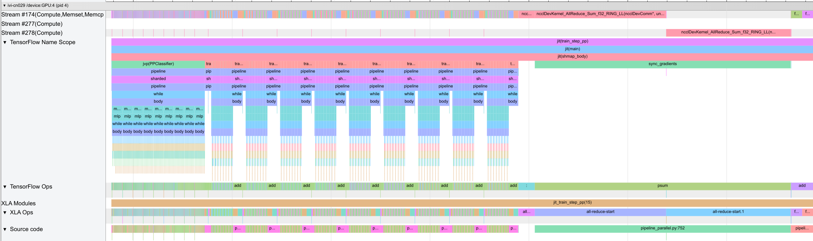
Compared to the previous networks, we see many small operations and scans, which are difficult to see all from the image above. If you want to dive deeper into the trace, you can download the trace and open it in TensorBoard. We find the expected pattern of the forward pass being an outer loop of 9 steps (8 microbatches + 1 pipeline shift slot), and each step containing the execution of the 8 layers per stage with communication. The backward pass is similar with 9 outer steps and 8 inner steps. Although the communication is not overlapped with the computation, the communication between stages only takes 17\(\mu{}s\) compared to 5ms of a single stage forward pass. Where a lot of time is lost, though, is in the gradient synchronization after the backward pass. Since the gradients only finish computing in the last microbatch step, we need to wait almost until the end before we can start communicating the gradients. This is a significant bottleneck in the non-looped pipeline, especially on hardware with high communication costs over the data axis. We also note that in Transformer models, we would see a slightly different pattern, since the activations are significantly larger (additional sequence length) and reduce the relative communication cost of the gradients. Further, we find a significant amount of time is spent in the dynamic_slice_update operation of the inner scan operation over layers, which suggests that we may get a significant speedup by removing the scan as in the single-GPU setup.

We now show the trace for the looped pipeline:

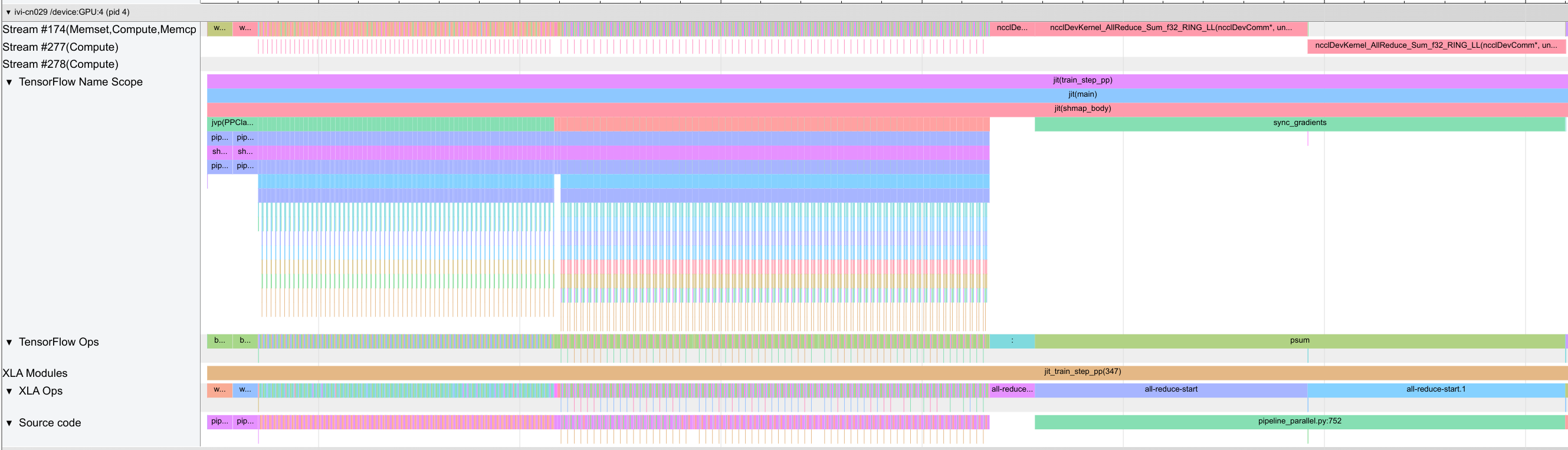
This trace has even more small operations, which we need to zoom in to see. We find the expected pattern of the forward pass being an outer loop of \(8 * 8 + 1=65\) steps, and each step containing the execution of only 1 layer. The backward pass is similar with 65 outer steps and 1 inner step. The communication again makes up only a small fraction of the total time, and the compiler overlaps the time with the scan operation computation. Still, we find a similar bottleneck in the gradient synchronization after the backward pass, which, in theory, the looping pipeline should be able to reduce. This is because the current implementation needs to stack the parameters over the looping axis within the pipeline, in order to support the SPMD jitting of the pipeline. Thus, the gradients are only communicated once the gradients for all parameters in the pipeline have been calculated. To obtain the maximum efficiency of the pipeline, we would need to support asynchronous gradient communication, which is left for future times. Nonetheless, already in its current version, the looping pipeline is 7% faster, taking 190ms for a full forward and backward pass versus 205ms for the non-looped pipeline.

Conclusion

In this notebook, we have discussed and implemented pipeline parallelism with micro-batching and looping pipelines. The main challenge of pipelines remains the pipeline bubble, which can reduce their efficiency. While looping pipelines and other strategies can improve its efficiency, we usually have to trade-off communication cost and computation time. Hence, the best trade-off depends on the specific model and hardware setup. We have also shown how to combine pipeline parallelism with data parallelism, and how to test the pipeline parallelism by comparing the outputs of the non-parallelized and parallelized model. For simplicity, we have not applied full sharding data parallelism, but the same principles apply and can be implemented without changes to the pipeline wrapper. We will show that in the final notebook on 3D parallelism. In the next notebook, we will discuss tensor parallelism, which is another strategy to parallelize the model across multiple devices.

References and Resources

[Huang et al., 2019] Huang, Y., Cheng, Y., Bapna, A., Firat, O., Chen, D., Chen, M., Lee, H., Ngiam, J., Le, Q.V. and Wu, Y., 2019. Gpipe: Efficient training of giant neural networks using pipeline parallelism. Advances in neural information processing systems, 32. Paper link

[Narayanan et al., 2021] Narayanan, D., Shoeybi, M., Casper, J., LeGresley, P., Patwary, M., Korthikanti, V., Vainbrand, D., Kashinkunti, P., Bernauer, J., Catanzaro, B. and Phanishayee, A., 2021, November. Efficient large-scale language model training on gpu clusters using megatron-lm. In Proceedings of the International Conference for High Performance Computing, Networking, Storage and Analysis (pp. 1-15). Paper link

[Lamy-Poirier, 2023] Lamy-Poirier, J., 2023. Breadth-First Pipeline Parallelism. Proceedings of Machine Learning and Systems, 5. Paper link

[McKinney, 2023] McKinney, A., 2023. A Brief Overview of Parallelism Strategies in Deep Learning. Blog post link

[Huggingface, 2024] Huggingface, 2024. Model Parallelism. Documentation link

[DeepSpeed, 2024] DeepSpeed, 2024. Pipeline Parallelism. Documentation link

---

If you found this tutorial helpful, consider ⭐-ing our repository.

For any questions, typos, or bugs that you found, please raise an issue on GitHub.

---