Part 5: Language Modeling with 3D Parallelism

Filled notebook:

Author: Phillip Lippe

In the previous tutorials, we have explored the concept of parallelism in the context of training large language models. We have seen how data parallelism can be used to distribute the training data across multiple devices, and how pipeline and tensor parallelism can be used to distribute the model across multiple devices. For training models with up to trillion parameters, one parallelism strategy alone will not be sufficient. Hence, in this tutorial, we will explore the concept of 3D parallelism, which combines data, pipeline, and tensor parallelism to train models like large language models (LLM).

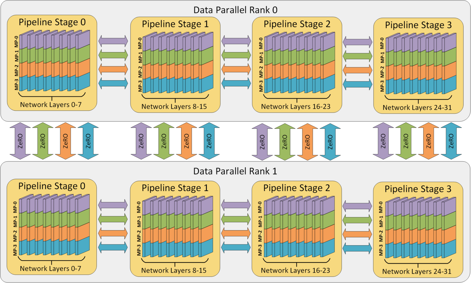
To combine all parallelism strategies, we need to create a three-dimensional mesh of devices. Each axis will correspond to one of our parallelism strategies. The data parallelism axis will be responsible for distributing the training data across devices, the pipeline parallelism axis will be responsible for distributing the model’s layers across devices, and the tensor parallelism axis will be responsible for parallelizing the individual layers across devices. Thereby, tensor parallelism requires the highest communication bandwidth, while data parallelism requires the lowest communication bandwidth. We need to take this communication bandwidth into account when designing the 3D parallelism mesh. For instance, GPUs that are within the same node and have a strong NVLink connection should be placed on the same tensor parallelism axis, while GPUs that are in different nodes should be placed on different tensor parallelism axes. Cross-node communication is much slower than the communication within a node, such that we may want to use data parallelism across nodes. Still, for nodes with a high communication bandwidth, we can use pipeline parallelism across nodes. This gives us the flexibility to design the 3D parallelism mesh according to the hardware we have available. An overview of the 3D parallelism mesh is shown in the figure below (figure credit: DeepSpeed, 2024).

In this notebook, we will combine the techniques we have implemented for data, pipeline and tensor parallelism to enable 3D parallelism. We demonstrate how easy it is in JAX to combine the different parallelism strategies, and experiment with different 3D parallelism configurations.

Prerequisites

First, let’s start with setting up the basic environment and utility functions we have seen from previous notebooks. We download the python scripts of the previous notebooks below. This is only needed when running on Google Colab, and local execution will skip this step automatically.

import os
import urllib.request
from urllib.error import HTTPError

# Github URL where python scripts are stored.
base_url = "https://raw.githubusercontent.com/phlippe/uvadlc_notebooks/master/docs/tutorial_notebooks/scaling/JAX/"
# Files to download.
python_files = [
    "single_gpu.py",
    "data_parallel.py",
    "pipeline_parallel.py",
    "tensor_parallel.py",
    "tensor_parallel_async.py",
    "tensor_parallel_transformer.py",
    "utils.py",
]
# For each file, check whether it already exists. If not, try downloading it.
for file_name in python_files:
    if not os.path.isfile(file_name):
        file_url = base_url + file_name
        print(f"Downloading {file_url}...")
        try:
            urllib.request.urlretrieve(file_url, file_name)
        except HTTPError as e:
            print(
                "Something went wrong. Please try to download the file directly from the GitHub repository, or contact the author with the full output including the following error:\n",
                e,
            )

As before, we simulate 8 devices on CPU to demonstrate the parallelism without the need for multiple GPUs or TPUs. If you are running on your local machine and have multiple GPUs available, you can comment out the lines below.

from utils import simulate_CPU_devices

simulate_CPU_devices()

We now import our standard libraries.

import functools
from pprint import pprint
from typing import Any, Callable, Dict, Tuple

import flax.linen as nn
import jax
import jax.numpy as jnp
import numpy as np
import optax
from jax.experimental.shard_map import shard_map
from jax.sharding import Mesh
from jax.sharding import PartitionSpec as P
from ml_collections import ConfigDict
from tqdm.auto import tqdm

PyTree = Any
Parameter = jax.Array | nn.Partitioned
Metrics = Dict[str, Tuple[jax.Array, ...]]

We also import the utility functions from the previous notebooks. Our notebook will rely on many concepts of previous tutorials, such as shard_module_params and sync_gradients for handling fully-sharded data parallelism, ModelParallelismWrapper and PipelineModule for handling pipeline parallelism, and the transformer blocks from the tensor parallelism notebook. If you are not familiar with these functions and modules, we recommend to go through the previous tutorials first.

from data_parallel import fold_rng_over_axis, shard_module_params, sync_gradients
from pipeline_parallel import ModelParallelismWrapper, PipelineModule
from single_gpu import (
    Batch,
    TrainState,
    accumulate_gradients,
    get_num_params,
    print_metrics,
)
from tensor_parallel_transformer import (
    TPInputEmbedding,
    TPTransformerBlock,
    TPTransformerParallelBlock,
    TransformerBackbone,
    split_array_over_mesh,
)

3D Parallelism

We will now combine the techniques we have implemented for data, pipeline and tensor parallelism to enable 3D parallelism. Most parallelization implementations we have done over the past tutorials have been designed with the idea that we may want to combine them in the future. For instance, the ModelParallelismWrapper supports nested model parallelism, where the module passed to the wrapper might also be partitioned over a different axis. Similarly, the PipelineModule operates independently of how the stages in the pipeline may be sharded. Moreover, our parameter sharding implementation in shard_module_params supports sharding over multiple axes at once, as we will see later on. All this together allows us to easily combine the different parallelism strategies.

Transformer Model

We start by implementing the transformer model that we will use for our 3D parallelism experiments. We will use the same transformer model as in the tensor parallelism tutorial, but slightly adjust it to also support pipeline parallelism. For this, we first write a wrapper around the transformer backbone, i.e. the scan over layers, such that we can pass it to the PipelineModule. It is the same technique as we have seen in the pipeline parallelism notebook. Note that for simplicity, we will not use looping pipelines here, but only a single pipeline stage. However, the implementation would easily allow for looping pipelines as well.

class PipelineTransformerBackbone(nn.Module):
    """Transformer backbone with pipeline and tensor parallelism.

    This module is a combination of the `TransformerBackbone` from the tensor parallelism tutorial
    and the `PipelineModule` from the pipeline parallelism tutorial.
    """

    config: ConfigDict
    train: bool
    mask: jax.Array | None = None
    block_fn: Any = TPTransformerBlock
    pipeline_module_class: Callable[..., nn.Module] = PipelineModule

    @nn.compact
    def __call__(self, x: jax.Array) -> jax.Array:
        axis_size = jax.lax.psum(1, self.config.pipeline_axis_name)
        # Define module per pipeline stage.
        stage_module_fn = functools.partial(
            TransformerBackbone,
            config=self.config,
            train=self.train,
            mask=self.mask,
            block_fn=self.block_fn,
            name="layers",
        )
        if axis_size == 1:
            # If pipeline axis size is 1, we don't need to define a pipeline module.
            module = stage_module_fn()
        else:
            # Define pipeline module.
            pipeline_module_fn = functools.partial(
                self.pipeline_module_class,
                model_axis_name=self.config.pipeline_axis_name,
                num_microbatches=self.config.num_microbatches,
                module_fn=stage_module_fn,
            )
            # Wrap pipeline module in parallelism wrapper over pipeline axis.
            # The tensor parallelism is handled within the TPTransformerBlock.
            module = ModelParallelismWrapper(
                module_fn=pipeline_module_fn,
                model_axis_name=self.config.pipeline_axis_name,
                name="pipeline",
            )
        x = module(x)
        return x

Another component we want to adjust is the output layer. In the tensor parallelism tutorial, we have changed our parallelization strategy from tensor to sequence parallelism, since the output requires the full softmax, i.e. full output size, and this may lead unnecessary replication of large tensors. In the 3d parallelism, we follow the same setup, but also add the pipeline parallel axis to the sequence parallelism. Essentially, from a mesh of (data, pipeline, tensor), we switch to (data, sequence) parallelism by combining the pipeline and tensor parallelism.

We first reorganize the input tensors by summing over the pipeline axis and splitting the output. We sum instead of gathering, since in pipeline parallelism, all devices except the last one will have zero’s in the output. Hence, summing across the pipeline axis is the equivalent to gathering and selecting only the output of the last stage. We then gather and split the data over the tensor axis as before. With that, each device across the joint pipeline and model axis will have a different subset of the input sequence.

To reduce the parameters per device, we apply parameter sharding as in Zero over the two axis. JAX supports axis names which are tuples of other axis names, such that we can shard over multiple axes at once. We will shard over the pipeline and tensor axis, such that each device will only have a subset of the parameters. We implement this below:

class TPPPOutputLayer(nn.Module):
    config: ConfigDict

    @nn.compact
    def __call__(self, x: jax.Array) -> jax.Array:
        # Pipeline outputs are zero's for all non-last stages.
        # Summing results results in all stages having the same, correct output.
        x = jax.lax.psum(x, axis_name=self.config.pipeline_axis_name)
        x = split_array_over_mesh(x, axis_name=self.config.pipeline_axis_name, split_axis=1)
        # Gather outputs over feature dimension and split over sequence length.
        x = jax.lax.all_gather(x, axis_name=self.config.model_axis_name, axis=-1, tiled=True)
        x = split_array_over_mesh(x, axis_name=self.config.model_axis_name, split_axis=1)
        # Shard parameters over model axis.
        norm_fn = shard_module_params(
            nn.RMSNorm,
            axis_name=(self.config.pipeline_axis_name, self.config.model_axis_name),
            min_weight_size=self.config.fsdp.min_weight_size,
        )
        dense_fn = shard_module_params(
            nn.Dense,
            axis_name=(self.config.pipeline_axis_name, self.config.model_axis_name),
            min_weight_size=self.config.fsdp.min_weight_size,
        )
        # Apply normalization and output layer.
        x = norm_fn(dtype=self.config.dtype, name="out_norm")(x)
        x = dense_fn(
            features=self.config.num_outputs,
            dtype=jnp.float32,
            name="output_layer",
        )(x)
        return x

Finally, we can combine everything together to create a Transformer model for 3D parallelism. Since every module requires different shardings in FSDP, we wrap each module below in its respective sharding. For instance, the input layer will receive the same input across the pipeline and tensor axis. We have already sharded the feature dimension over the tensor axis, such that the remaining parameter axes can be sharded over the data and pipeline axis jointly. We perform the same computation over the pipeline axis in the input layer, but since it only consists of an embedding lookup and adding of positional encoding, its computation is negligible.

The transformer backbone will then process via a pipeline process, with each stage additionally sharded over the tensor axis. In FSDP, we can shard the parameters additionally over the data axis.

Finally, the output layer already shards its parameters over the pipeline and tensor axis. Thus, we only need to shard them additionally over the data axis in FSDP.

A small note on our FSDP implementation: for simplicity, we enforce each application of shard_module_params to look for parameter axis that have been unsharded before. This is not strictly necessary, as we already support shard_module_params to shard over multiple axes at once. For large arrays with few axes, like the input embeddings, it may be beneficial to support the double sharding in some cases. However, it simplifies the implementation and is sufficient for our purposes here.

class Transformer(nn.Module):
    config: ConfigDict
    block_fn: Any = TPTransformerBlock

    @nn.compact
    def __call__(self, x: jax.Array, train: bool, mask: jax.Array | None = None) -> jax.Array:
        if mask is None and self.config.causal_mask:
            mask = nn.make_causal_mask(x[0:1], dtype=jnp.bool_)
        # Input embedding. Replicated across pipeline axis.
        input_layer = TPInputEmbedding
        if "Embed" in self.config.fsdp.modules:
            input_layer = shard_module_params(
                input_layer,
                axis_name=(self.config.data_axis_name, self.config.pipeline_axis_name),
                min_weight_size=self.config.fsdp.min_weight_size,
            )
        x = input_layer(
            config=self.config,
            name="input_embedding",
        )(x)
        # Backbone.
        backbone_layer = PipelineTransformerBackbone
        if "Backbone" in self.config.fsdp.modules:
            backbone_layer = shard_module_params(
                backbone_layer,
                axis_name=self.config.data_axis_name,
                min_weight_size=self.config.fsdp.min_weight_size,
            )
        x = backbone_layer(
            config=self.config,
            train=train,
            mask=mask,
            block_fn=self.block_fn,
            name="backbone",
        )(x)
        # Output layer.
        output_layer = TPPPOutputLayer
        if "Output" in self.config.fsdp.modules:
            output_layer = shard_module_params(
                output_layer,
                axis_name=self.config.data_axis_name,
                min_weight_size=self.config.fsdp.min_weight_size,
            )
        x = output_layer(
            config=self.config,
            name="output_layer",
        )(x)
        return x

And that’s it. We have now implemented a transformer model that supports 3D parallelism with few adjustments from the original tensor-parallel model. We can set up the training of the model.

Initialization

We start by defining the config for our model. Since the notebook is supposed to also run on CPU, we choose a very small model here. However, on actual multi-accelerator hardware, we would scale up the model considerably. Feel free to test out different configurations.

data_config = ConfigDict(
    dict(
        batch_size=32,
        vocab_size=100,
        seq_len=8,
    )
)
fsdp = ConfigDict(
    dict(
        modules=("Embed", "Backbone", "Output"),
        axis_name="data",
        min_weight_size=2**8,
    )
)
model_config = ConfigDict(
    dict(
        hidden_size=256,
        dropout_rate=0.1,
        mlp_expansion=4,
        num_layers=6,
        head_dim=32,
        normalize_qk=True,
        positional_encoding_type="learned",
        parallel_block=True,
        causal_mask=True,
        vocab_size=data_config.vocab_size,
        num_outputs=data_config.vocab_size,
        dtype=jnp.bfloat16,
        data_axis_name="data",
        model_axis_name="tensor",
        model_axis_size=2,
        pipeline_axis_name="pipe",
        pipeline_axis_size=2,
        num_microbatches=8,
        remat=("Block",),
        fsdp=fsdp,
    )
)
model_config.num_heads = model_config.hidden_size // model_config.head_dim
model_config.num_layers //= model_config.pipeline_axis_size
optimizer_config = ConfigDict(
    dict(
        learning_rate=2e-4,
        num_minibatches=1,
    )
)
config = ConfigDict(
    dict(
        model=model_config,
        optimizer=optimizer_config,
        data=data_config,
        data_axis_name=model_config.data_axis_name,
        model_axis_name=model_config.model_axis_name,
        model_axis_size=model_config.model_axis_size,
        pipeline_axis_name=model_config.pipeline_axis_name,
        pipeline_axis_size=model_config.pipeline_axis_size,
        seed=42,
    )
)

We start by creating our device mesh. We will have three axis this time, which split the devices into a 2x2x2 grid (for 8 devices). The closest devices are on the same tensor axis (e.g. 0 and 1), the next closest devices are on the same pipeline axis (e.g. 0 and 2), and the last axis is the data parallel axis (e.g. 0 and 4). For your actual hardware, you should adjust the device order/mesh to optimally fit your communication hardware. On GPUs, you can find your NVLink connections with nvidia-smi topo -m.

device_array = np.array(jax.devices()).reshape(
    -1, config.pipeline_axis_size, config.model_axis_size
)
mesh = Mesh(
    device_array, (config.data_axis_name, config.pipeline_axis_name, config.model_axis_name)
)
mesh

2024-03-07 10:49:34.624870: E external/xla/xla/stream_executor/cuda/cuda_driver.cc:273] failed call to cuInit: CUDA_ERROR_NO_DEVICE: no CUDA-capable device is detected
CUDA backend failed to initialize: FAILED_PRECONDITION: No visible GPU devices. (Set TF_CPP_MIN_LOG_LEVEL=0 and rerun for more info.)

Mesh(device_ids=array([[[0, 1],
        [2, 3]],

       [[4, 5],
        [6, 7]]]), axis_names=('data', 'pipe', 'tensor'))

We next create the transformer module. There is nothing special about it, besides that we do not need to wrap it in a shard_module_wrapper since we already shard parameters within the model.

def get_transformer_module(config: ConfigDict):
    block_fn = TPTransformerParallelBlock if config.parallel_block else TPTransformerBlock
    return Transformer(config=config, block_fn=block_fn)


model_transformer = get_transformer_module(config=config.model)

We then create the optimizer. Again, we use the same exponential decay schedule with warmup as for the other tutorials, although for an actual training, you may want to consider other alternatives as well, like LAMB or AdamW.

optimizer_transformer = optax.adam(
    learning_rate=optax.warmup_exponential_decay_schedule(
        init_value=0,
        peak_value=config.optimizer.learning_rate,
        warmup_steps=10,
        transition_steps=1,
        decay_rate=0.99,
    )
)

For this notebook, we still with our random token dataset, but you can replace it with any other dataset you like.

rng = jax.random.PRNGKey(config.seed)
model_init_rng, data_inputs_rng = jax.random.split(rng)

tokens = jax.random.randint(
    data_inputs_rng,
    (config.data.batch_size, config.data.seq_len),
    1,
    config.data.vocab_size,
)
batch_transformer = Batch(
    inputs=jnp.pad(tokens[:, :-1], ((0, 0), (1, 0)), constant_values=0),
    labels=tokens,
)

The initialization function is again the same as in the previous tutorials, and all parameter shardings are handled automatically.

def init_transformer(rng: jax.random.PRNGKey, x: jax.Array) -> TrainState:
    init_rng, rng = jax.random.split(rng)
    variables = model_transformer.init({"params": init_rng}, x, train=False)
    params = variables.pop("params")
    state = TrainState.create(
        apply_fn=model_transformer.apply,
        params=params,
        tx=optimizer_transformer,
        rng=rng,
    )
    return state

We first infer the partitioning for each parameter below.

init_transformer_fn = jax.jit(
    shard_map(
        init_transformer,
        mesh,
        in_specs=(P(), P(config.data_axis_name)),
        out_specs=P(),
        check_rep=False,
    ),
)
state_transformer_shapes = jax.eval_shape(
    init_transformer_fn, model_init_rng, batch_transformer.inputs
)
state_transformer_specs = nn.get_partition_spec(state_transformer_shapes)

Let’s check the partitioning and shapes of the parameters, to see if the sharding has been done correctly and understand the setup. We first extract the shapes, which are per-device since the out-specification is P() for now.

param_shapes = jax.tree_map(
    lambda x: x.value.shape if hasattr(x, "value") else x.shape,
    state_transformer_shapes.params,
    is_leaf=lambda x: isinstance(x, nn.Partitioned),
)

For the input layer, we find the following shapes:

print("Input Embedding")
pprint(state_transformer_specs.params["input_embedding"])
print("Per-device shapes")
pprint(param_shapes["input_embedding"])

Input Embedding
{'module': {'sharded': {'pos_enc': {'pos_emb': PartitionSpec('tensor', None, ('data', 'pipe'))},
                        'token_emb': {'embedding': PartitionSpec('tensor', None, ('data', 'pipe'))}}}}
Per-device shapes
{'module': {'sharded': {'pos_enc': {'pos_emb': (1, 8, 32)},
                        'token_emb': {'embedding': (1, 100, 32)}}}}

Both the positional encoding and embedding are split over the tensor axis, which results in the first axis being 1 per device and partitioned over tensor. The last axis is the feature dimension, which is 256 globally, but 128 after the split over the tensor axis. This axis is sharded over data and pipe, which results in 32 per device (4 devices over the joint axis).

print("Output Layer")
pprint(state_transformer_specs.params["output_layer"])
print("Per-device shapes")
pprint(param_shapes["output_layer"])

Output Layer
{'out_norm': {'scale': PartitionSpec()},
 'output_layer': {'bias': PartitionSpec(),
                  'kernel': PartitionSpec(('pipe', 'tensor'), 'data')}}
Per-device shapes
{'out_norm': {'scale': (256,)},
 'output_layer': {'bias': (100,), 'kernel': (64, 50)}}

The output layer has the norm and bias replicated over all devices, since in our configuration for the CPU, both of the tensors are very small and below the sharding threshold. The kernel weights are sharded over pipe and tensor on the first axis, which is the largest and originally 256, which results in 32 per device (4 devices over the joint axis). We additionally shard the last axis over data, which results in 50 per device (2 devices over the axis with 100 outputs).

For the transformer backbone, we first look at the input layer of the parallel block. Since the tensor parallelism introduces multiple identical sublayers (shards), we only look at shard_0 for simplicity. Note that if you are using the sequential block, the lines below need to be adjusted accordingly.

print("Transformer Backbone - HQKV")
pprint(
    state_transformer_specs.params["backbone"]["pipeline"]["sharded"]["layers"]["block"]["hqkv"][
        "shard_0"
    ]["sharded"]
)
print("Per-device shapes")
pprint(
    param_shapes["backbone"]["pipeline"]["sharded"]["layers"]["block"]["hqkv"]["shard_0"][
        "sharded"
    ]
)

Transformer Backbone - HQKV
{'mlp': {'dense': {'bias': PartitionSpec('pipe', None, 'tensor', 'data'),
                   'kernel': PartitionSpec('pipe', None, 'tensor', None, 'data')}},
 'qkv': {'key': {'kernel': PartitionSpec('pipe', None, 'tensor', 'data', None, None)},
         'key_norm': {'scale': PartitionSpec('pipe', None, 'tensor', None)},
         'query': {'kernel': PartitionSpec('pipe', None, 'tensor', 'data', None, None)},
         'query_norm': {'scale': PartitionSpec('pipe', None, 'tensor', None)},
         'value': {'kernel': PartitionSpec('pipe', None, 'tensor', 'data', None, None)}}}
Per-device shapes
{'mlp': {'dense': {'bias': (1, 3, 1, 256), 'kernel': (1, 3, 1, 128, 256)}},
 'qkv': {'key': {'kernel': (1, 3, 1, 64, 4, 32)},
         'key_norm': {'scale': (1, 3, 1, 32)},
         'query': {'kernel': (1, 3, 1, 64, 4, 32)},
         'query_norm': {'scale': (1, 3, 1, 32)},
         'value': {'kernel': (1, 3, 1, 64, 4, 32)}}}

All parameters share the first three axes: pipeline device stacking (sharded over pipe), number of layer per pipeline stage (3 per device), and tensor device stacking (sharded over tensor). After that, we have the individual parameter shapes. For the MLP, the bias and kernel increase the feature size to 1024. This is split over the tensor axis, and sharded over the data axis (hence 1/4 of the feature size per device). The input axis of the kernel is split over different tensor shards, hence 1/2 of the original 256 feature dimension.

For the key, query and value layers, we have the input size of 256, which is split over the tensor axis and sharded over the data axis. The output size is (4, 32) per device, since the head dimension is 32 and the number of heads is 8, split over the tensor axis (hence 1/2 of the head count per device).

print("Transformer Backbone - Output")
pprint(
    state_transformer_specs.params["backbone"]["pipeline"]["sharded"]["layers"]["block"]["out"][
        "shard_0"
    ]["sharded"]
)
print("Per-device shapes")
pprint(
    param_shapes["backbone"]["pipeline"]["sharded"]["layers"]["block"]["out"]["shard_0"]["sharded"]
)

Transformer Backbone - Output
{'attn': {'out': {'bias': PartitionSpec('pipe', None, 'tensor', 'data'),
                  'kernel': PartitionSpec('pipe', None, 'tensor', None, None, 'data')}},
 'mlp': {'dense': {'bias': PartitionSpec('pipe', None, 'tensor', 'data'),
                   'kernel': PartitionSpec('pipe', None, 'tensor', 'data', None)}}}
Per-device shapes
{'attn': {'out': {'bias': (1, 3, 1, 64), 'kernel': (1, 3, 1, 4, 32, 64)}},
 'mlp': {'dense': {'bias': (1, 3, 1, 64), 'kernel': (1, 3, 1, 256, 128)}}}

On the output side of the transformer backbone, we have the same first three axes. The output kernel of the MLP model is the mirror image of the input size. The attention output kernel is of size (4, 32, 64), where the first is again the number of heads per device, 32 the head dimension, and 64 the feature dimension split over both the tensor and data axis.

With that, the sharding of the parameters appears to be correct. We can now proceed to fully initialize the model.

init_transformer_fn = jax.jit(
    shard_map(
        init_transformer,
        mesh,
        in_specs=(P(), P(config.data_axis_name)),
        out_specs=state_transformer_specs,
        check_rep=False,
    ),
)
state_transformer = init_transformer_fn(model_init_rng, batch_transformer.inputs)
print(f"Number of parameters: {get_num_params(state_transformer):_}")

Number of parameters: 4_784_484

The model is now fully initialized and ready for training. We can now proceed to the training loop.

Training

The loss function will be the same as in the previous tensor parallelism tutorial, with small modifications to introduce the pipeline parallelism. On the input side, we split the dropout RNG also over the pipeline axis. This gives us a different RNG per device. On the output side, we need to find the labels that correspond to the correct output slice per device. We use again the split_array_over_mesh function to subselect the array over the sequence length axis. We then compute the loss as before.

def loss_fn(
    params: PyTree,
    apply_fn: Any,
    batch: Batch,
    rng: jax.Array,
) -> Tuple[jax.Array, Dict[str, Any]]:
    # Since dropout masks vary across the batch dimension, we want each device to generate a
    # different mask. We can achieve this by folding the rng over the data axis, so that each
    # device gets a different rng and thus mask.
    dropout_rng = fold_rng_over_axis(
        rng, (config.data_axis_name, config.pipeline_axis_name, config.model_axis_name)
    )
    # Remaining computation is the same as before for single device.
    logits = apply_fn(
        {"params": params},
        batch.inputs,
        train=True,
        rngs={"dropout": dropout_rng},
    )
    # Select the labels per device.
    labels = batch.labels
    labels = split_array_over_mesh(labels, axis_name=config.pipeline_axis_name, split_axis=1)
    labels = split_array_over_mesh(labels, axis_name=config.model_axis_name, split_axis=1)
    assert (
        logits.shape[:-1] == labels.shape
    ), f"Logits and labels shapes do not match: {logits.shape} vs {labels.shape}"
    loss = optax.softmax_cross_entropy_with_integer_labels(logits, labels)
    correct_pred = jnp.equal(jnp.argmax(logits, axis=-1), labels)
    batch_size = np.prod(labels.shape)
    # Collect metrics and return loss.
    step_metrics = {
        "loss": (loss.sum(), batch_size),
        "accuracy": (correct_pred.sum(), batch_size),
    }
    loss = loss.mean()
    return loss, step_metrics

The training step is similarly adjusted. The gradients and the metrics are synced over all three axes. The rest of the training loop is the same as in the previous tutorials.

def train_step(
    state: TrainState,
    metrics: Metrics | None,
    batch: Batch,
) -> Tuple[TrainState, Metrics]:
    rng, step_rng = jax.random.split(state.rng)
    grads, step_metrics = accumulate_gradients(
        state,
        batch,
        step_rng,
        config.optimizer.num_minibatches,
        loss_fn=loss_fn,
    )
    # Update parameters. We need to sync the gradients across devices before updating.
    with jax.named_scope("sync_gradients"):
        grads = sync_gradients(
            grads, (config.data_axis_name, config.pipeline_axis_name, config.model_axis_name)
        )
    new_state = state.apply_gradients(grads=grads, rng=rng)
    # Sum metrics across replicas. Alternatively, we could keep the metrics separate
    # and only synchronize them before logging. For simplicity, we sum them here.
    with jax.named_scope("sync_metrics"):
        step_metrics = jax.tree_map(
            lambda x: jax.lax.psum(
                x,
                axis_name=(
                    config.data_axis_name,
                    config.pipeline_axis_name,
                    config.model_axis_name,
                ),
            ),
            step_metrics,
        )
    if metrics is None:
        metrics = step_metrics
    else:
        metrics = jax.tree_map(jnp.add, metrics, step_metrics)
    return new_state, metrics

We are now ready to train our model. We shard the input batch over the data axis, and set the sharding specification as we have inferred during the initialization. Note that if we would run over multiple nodes/hosts and devices across the tensor or pipeline axis have different hosts, we may have difficulties to synchronize the hosts to input the same batch over the two parallelization axes. Alternatively, we can adjust the data input sharding to shard over all axes, and gather the input batch over the tensor and pipeline axis before starting our training step. However, for simplicity, we assume that all devices are on the same host in this notebook.

train_step_fn = jax.jit(
    shard_map(
        train_step,
        mesh,
        in_specs=(state_transformer_specs, P(), P(config.data_axis_name)),
        out_specs=(state_transformer_specs, P()),
        check_rep=False,
    ),
    donate_argnames=("state", "metrics"),
)
_, metric_shapes = jax.eval_shape(
    train_step_fn,
    state_transformer,
    None,
    batch_transformer,
)
metrics_transformer = jax.tree_map(lambda x: jnp.zeros(x.shape, dtype=x.dtype), metric_shapes)
state_transformer, metrics_transformer = train_step_fn(
    state_transformer, metrics_transformer, batch_transformer
)

/home/plippe/anaconda3/envs/jax/lib/python3.10/site-packages/jax/_src/interpreters/mlir.py:761: UserWarning: Some donated buffers were not usable: ShapedArray(float32[1,3,1,256]), ShapedArray(float32[1,3,1,128,256]), ShapedArray(float32[1,3,1,64,4,32]), ShapedArray(float32[1,3,1,32]), ShapedArray(float32[1,3,1,64,4,32]), ShapedArray(float32[1,3,1,32]), ShapedArray(float32[1,3,1,64,4,32]), ShapedArray(float32[1,3,1,128,256]), ShapedArray(float32[1,3,1,64,4,32]), ShapedArray(float32[1,3,1,32]), ShapedArray(float32[1,3,1,64,4,32]), ShapedArray(float32[1,3,1,32]), ShapedArray(float32[1,3,1,64,4,32]), ShapedArray(float32[1,3,1,64]), ShapedArray(float32[1,3,1,4,32,64]), ShapedArray(float32[1,3,1,64]), ShapedArray(float32[1,3,1,256,128]), ShapedArray(float32[1,3,1,4,32,64]), ShapedArray(float32[1,3,1,256,128]), ShapedArray(float32[1,3,1,64]), ShapedArray(float32[1,8,32]), ShapedArray(float32[1,100,32]), ShapedArray(float32[64,50]), ShapedArray(float32[1,3,1,256]), ShapedArray(float32[1,3,1,128,256]), ShapedArray(float32[1,3,1,64,4,32]), ShapedArray(float32[1,3,1,32]), ShapedArray(float32[1,3,1,64,4,32]), ShapedArray(float32[1,3,1,32]), ShapedArray(float32[1,3,1,64,4,32]), ShapedArray(float32[1,3,1,128,256]), ShapedArray(float32[1,3,1,64,4,32]), ShapedArray(float32[1,3,1,32]), ShapedArray(float32[1,3,1,64,4,32]), ShapedArray(float32[1,3,1,32]), ShapedArray(float32[1,3,1,64,4,32]), ShapedArray(float32[1,3,1,64]), ShapedArray(float32[1,3,1,4,32,64]), ShapedArray(float32[1,3,1,64]), ShapedArray(float32[1,3,1,256,128]), ShapedArray(float32[1,3,1,4,32,64]), ShapedArray(float32[1,3,1,256,128]), ShapedArray(float32[1,3,1,64]), ShapedArray(float32[1,8,32]), ShapedArray(float32[1,100,32]), ShapedArray(float32[64,50]), ShapedArray(float32[1,3,1,256]), ShapedArray(float32[1,3,1,128,256]), ShapedArray(float32[1,3,1,64,4,32]), ShapedArray(float32[1,3,1,32]), ShapedArray(float32[1,3,1,64,4,32]), ShapedArray(float32[1,3,1,32]), ShapedArray(float32[1,3,1,64,4,32]), ShapedArray(float32[1,3,1,128,256]), ShapedArray(float32[1,3,1,64,4,32]), ShapedArray(float32[1,3,1,32]), ShapedArray(float32[1,3,1,64,4,32]), ShapedArray(float32[1,3,1,32]), ShapedArray(float32[1,3,1,64,4,32]), ShapedArray(float32[1,3,1,64]), ShapedArray(float32[1,3,1,4,32,64]), ShapedArray(float32[1,3,1,64]), ShapedArray(float32[1,3,1,256,128]), ShapedArray(float32[1,3,1,4,32,64]), ShapedArray(float32[1,3,1,256,128]), ShapedArray(float32[1,3,1,64]), ShapedArray(float32[1,8,32]), ShapedArray(float32[1,100,32]), ShapedArray(float32[64,50]).
See an explanation at https://jax.readthedocs.io/en/latest/faq.html#buffer-donation.
  warnings.warn("Some donated buffers were not usable:"

Finally, we run the model for a few steps. Feel free to adjust the number of steps. We will not run the model for a long time, since we are running on CPU and the model is very small. However, on actual multi-accelerator hardware, you can scale up the model and run for a longer time.

for _ in tqdm(range(20)):
    state_transformer, metrics_transformer = train_step_fn(
        state_transformer, metrics_transformer, batch_transformer
    )
final_metrics_transformer = jax.tree_map(
    lambda x: jnp.zeros(x.shape, dtype=x.dtype), metric_shapes
)
state_transformer, final_metrics_transformer = train_step_fn(
    state_transformer, final_metrics_transformer, batch_transformer
)
print_metrics(final_metrics_transformer, title="Final Metrics - Transformer")

 Final Metrics - Transformer
accuracy: 0.855469
loss: 1.063429

The model achieves similar results as in the previous tutorials, but may be slightly lower due to the small sequence length (by default 8). You can increase the sequence length to get better results, but keep in mind that the memory requirements will increase as well.

Profiling

As a final step, we can profile a larger model to see the performance of the 3D parallelism and compare different configurations. We recreate the model from the tensor parallelism tutorial with around 1 billion parameters. We use the same input batch size of 128, sequence length 1024, and vocabulary size 32k. We run the experiments on a single node with 8 A5000 GPUs, each having 24GB memory and having an NVLink between pairs of GPUs with 60GB/s communication bandwidth.

We first use the same 3D parallelism configuration as in the config up, using a 2x2x2 grid. We then profile the model and find a step time of 2.9 seconds. This is slower than the pure tensor parallelism model at 2.6 seconds. This is because the pipeline axis adds additional communication between devices, which are not well connected in our system and requires an additional microbatch of compute. In terms of memory, we only use 8.5GB per device, which is well within the 24GB memory of the A5000:

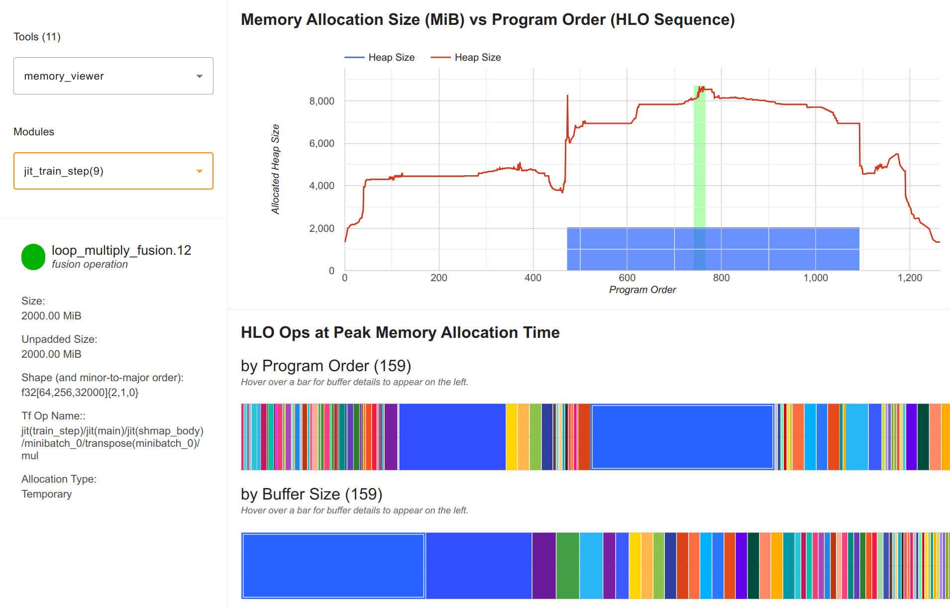
The largest array are the output logits of size (64, 256, 32000) (batch size 128 split over 2 data devices, sequence length 1024 split over 4 tensor and pipeline devices). Further, it is in float32 precision for numerical stability, which results in 2GB per device for this single array. The other arrays are much smaller and well within the memory limits. This highlights the importance of switching the parallelism strategies in the output to reduce the memory requirements.

Nonetheless, using only 1/3 of our available GPU memory indicates that we can either scale up the model, or use techniques that speed up the training for larger memory usage. For instance, we can disable parameter sharding over the data axis, which increases the per-device memory usage since all parameters are replicated now. If we use a 4x1x2 grid (4 data, 1 pipeline, 2 tensor devices), we have 500 million parameters per device (1 billion parameters in total over the two tensor devices), which requires roughly 6GB extra memory per device. We profile the memory usage below:

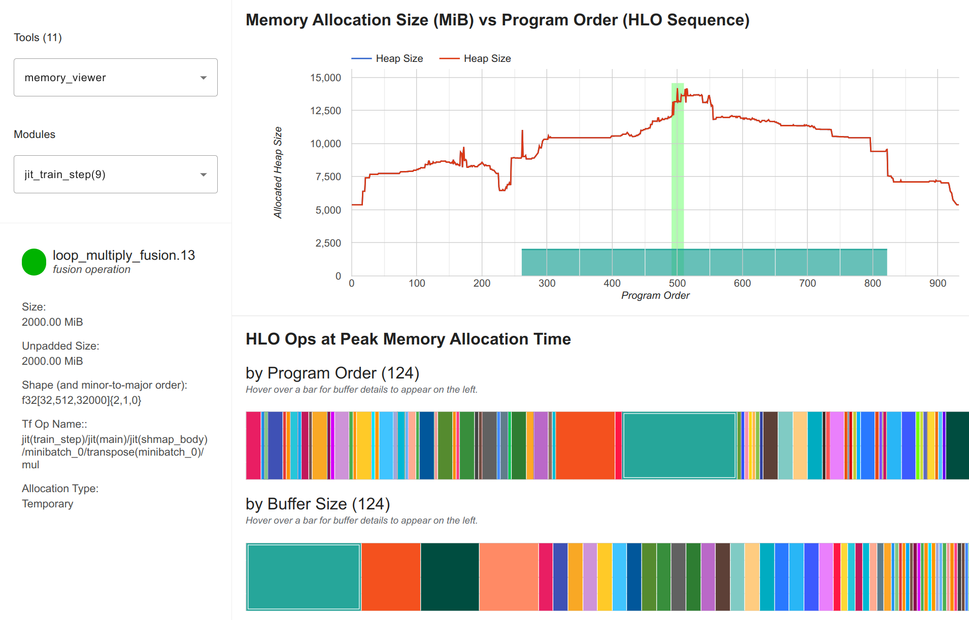
Each device now uses 14.5GB, which is still within the 24GB memory of the A5000. The largest array is still the output logits, but more parameter and optimizer state arrays are on each device, as seen by the higher initial memory usage. Without FSDP, we reduce the communication needed over devices, and we have a step time of 2.5 seconds now. This is slightly faster than the 3D parallelism with FSDP, but we may want to use the memory for increased batch sizes or rematting fewer layers. In the end, the best configuration depends on the specific hardware at hand, and the requirements we have from the training (e.g. minimum batch size, sequence length, etc.).

Conclusion

In this tutorial, we have combined the techniques we have implemented for data, pipeline and tensor parallelism to enable 3D parallelism. We have seen how easy it is in JAX to combine the different parallelism strategies using our previous implementations, and experiment with different 3D parallelism configurations. We have also seen how to profile the performance of the 3D parallelism and compare different configurations.

With that, we conclude our tutorial series on parallelism in JAX. We hope you have gained a good understanding of the different parallelism strategies and how to implement them in JAX. We hope you have enjoyed the tutorials and learned something new. If you have any questions or feedback, feel free to reach out or create an issue on our GitHub repository. Happy scaling!

References and Resources

[Shoeybi et al., 2019] Shoeybi, M., Patwary, M., Puri, R., LeGresley, P., Casper, J. and Catanzaro, B., 2019. Megatron-lm: Training multi-billion parameter language models using model parallelism. arXiv preprint arXiv:1909.08053. Paper link

[Hagemann et al., 2023] Hagemann, J., Weinbach, S., Dobler, K., Schall, M. and de Melo, G., 2023, October. Efficient Parallelization Layouts for Large-Scale Distributed Model Training. In Workshop on Advancing Neural Network Training: Computational Efficiency, Scalability, and Resource Optimization (WANT@ NeurIPS 2023). Paper link

[Huggingface, 2024] Huggingface, 2024. Model Parallelism. Documentation link

[DeepSpeed, 2024] DeepSpeed, 2024. Pipeline Parallelism. Tutorial link

---

If you found this tutorial helpful, consider ⭐-ing our repository.

For any questions, typos, or bugs that you found, please raise an issue on GitHub.

---