Part 4.3: Transformers with Tensor Parallelism
Filled notebook: 
![]()
Author: Phillip Lippe
In the previous two parts on tensor parallelism, we have seen how to parallelize simple models across multiple GPUs. In this part, we will see how to parallelize a transformer model across multiple GPUs. Transformer models are a common use case for tensor parallelism, as they are widely used in large-scale models for natural language processing and computer vision. For instance, it is the key architecture in GPT-4, Gemini, PALM, and ViT-22b. Hence, we will review the specific challenges of parallelizing transformers, how to address them, and how to maximize the efficiency of the parallelization. In the end, we will profile a 1-billion parameter model on 8 GPUs and discuss potential bottlenecks remaining.
Prerequisites
First, let’s start with setting up the basic environment and utility functions we have seen from previous notebooks. We download the python scripts of the previous notebooks below. This is only needed when running on Google Colab, and local execution will skip this step automatically.
[1]:
import os
import urllib.request
from urllib.error import HTTPError

# Github URL where python scripts are stored.
base_url = "https://raw.githubusercontent.com/phlippe/uvadlc_notebooks/master/docs/tutorial_notebooks/scaling/JAX/"
# Files to download.
python_files = [
    "single_gpu.py",
    "data_parallel.py",
    "pipeline_parallel.py",
    "tensor_parallel.py",
    "tensor_parallel_async.py",
    "utils.py",
]
# For each file, check whether it already exists. If not, try downloading it.
for file_name in python_files:
    if not os.path.isfile(file_name):
        file_url = base_url + file_name
        print(f"Downloading {file_url}...")
        try:
            urllib.request.urlretrieve(file_url, file_name)
        except HTTPError as e:
            print(
                "Something went wrong. Please try to download the file directly from the GitHub repository, or contact the author with the full output including the following error:\n",
                e,
            )
As before, we simulate 8 devices on CPU to demonstrate the parallelism without the need for multiple GPUs or TPUs. If you are running on your local machine and have multiple GPUs available, you can comment out the lines below.
[2]:
from utils import simulate_CPU_devices

simulate_CPU_devices()
We now import our standard libraries.
[3]:
import functools
from pprint import pprint
from typing import Any, Callable, Dict, Tuple

import flax.linen as nn
import jax
import jax.numpy as jnp
import numpy as np
import optax
from jax.experimental.shard_map import shard_map
from jax.sharding import Mesh
from jax.sharding import PartitionSpec as P
from ml_collections import ConfigDict
from tqdm.auto import tqdm

PyTree = Any
Parameter = jax.Array | nn.Partitioned
Metrics = Dict[str, Tuple[jax.Array, ...]]
We also import the utility functions from the previous notebooks. Our notebook will rely on the ModelParallelismWrapper from the pipeline parallelism notebook. If you are not familiar with it, it is recommended to look at the implementation of this module before continuing.
[4]:
from data_parallel import fold_rng_over_axis, shard_module_params
from pipeline_parallel import ModelParallelismWrapper
from single_gpu import Batch, TrainState, get_num_params, print_metrics
from tensor_parallel import MLPBlockInput, MLPBlockOutput, train_step_tp
from tensor_parallel_async import TPAsyncDense, TPAsyncMLPBlock, TPNorm
Tensor Parallelism in Transformer Models
In this section, we will implement a transformer model with tensor parallelism and fully-sharded data parallelism. We will use the same async linear layer as before, but extend it to the full transformer model, including the attention layers. In that, we show common implementation strategies in tensor parallelism for transformers specifically.
Attention Layer
The attention layer is the key component of the transformer model, and is used to model the interactions between different input tokens. It consists of a query, key, and value projection, followed by a scaled dot-product attention, and a final linear layer. The computation graph of the attention layer is visualized below (figure credit - Vaswani et al., 2017).

Splitting the query, key and value over hidden dimension would require several communications between devices, since all hidden dimensions are needed for calculating the attention scores. This would be inefficient, and we would like to avoid it if possible. Instead, we can exploit another key aspect of the attention layers in transformer models: multi-head attention. In multi-head attention, we project the input features into multiple heads, and perform the attention computation independently on each head. We then concatenate the outputs of each head, and project the concatenated output back to the original feature size. To reduce communication, we therefore split the attention calculation over the heads across devices, and only need to communicate the original input and the output of the individual heads. This becomes very similar to the MLP block we implemented earlier, and we can use the same async linear layers to implement the attention layer.
Let’s start with implementing the input layer. We first need to project the input features into the query, key, and value space, which we do with individual linear layer. The DenseGeneral layer allows us to directly output the reshaped array of [..., num_heads, head_dim] instead of a manual reshape. Following PALM and ViT-22b, we do not apply a bias term to the projection layers. Further, the ViT-22b model normalizes the query and key features before the attention computation. This
prevents instability at large scale where the attention logits can become very large and cause a close-to one-hot attention distribution very early in the training. We adopt this normalization in our implementation below.
[5]:
class QKVDense(nn.Module):
    config: ConfigDict
    num_heads: int
    head_dim: int
    kernel_init: Callable
    use_bias: bool = False

    @nn.compact
    def __call__(self, x: jax.Array) -> Tuple[jax.Array, jax.Array, jax.Array]:
        q = nn.DenseGeneral(
            (self.num_heads, self.head_dim),
            kernel_init=self.kernel_init,
            use_bias=False,
            dtype=self.config.dtype,
            name="query",
        )(x)
        k = nn.DenseGeneral(
            (self.num_heads, self.head_dim),
            kernel_init=self.kernel_init,
            use_bias=False,
            dtype=self.config.dtype,
            name="key",
        )(x)
        v = nn.DenseGeneral(
            (self.num_heads, self.head_dim),
            kernel_init=self.kernel_init,
            use_bias=False,
            dtype=self.config.dtype,
            name="value",
        )(x)

        if self.config.normalize_qk:
            q = nn.RMSNorm(
                dtype=self.config.dtype,
                name="query_norm",
            )(q)
            k = nn.RMSNorm(
                dtype=self.config.dtype,
                name="key_norm",
            )(k)
        return q, k, v
Since each device will calculate an independent set of heads, the dot product attention does not need to parallelized. Instead, we can simply reuse our implementation from the first notebook for single-GPU usage, where we adjusted the attention calculation to higher precision for numerical stability of the attention softmax.
[6]:
def dot_product_attention(
    query: jax.Array,
    key: jax.Array,
    value: jax.Array,
    mask: jax.Array | None,
    softmax_dtype: jnp.dtype = jnp.float32,
):
    """Dot-product attention.

    Follows the setup of https://flax.readthedocs.io/en/latest/api_reference/flax.linen/layers.html#flax.linen.dot_product_attention,
    but supports switch to float32 for numerical stability during softmax.

    Args:
        query: The query array, shape [..., num queries, num heads, hidden size].
        key: The key array, shape [..., num keys, num heads, hidden size].
        value: The value array, shape [..., num keys, num heads, hidden size].
        mask: The boolean mask array (0 for masked values, 1 for non-masked). If None, no masking is applied.
        softmax_dtype: The dtype to use for the softmax operation.

    Returns:
        The attention output array, shape [..., num queries, num heads, hidden size].
    """
    num_features = query.shape[-1]
    dtype = query.dtype
    scale = num_features**-0.5
    query = query * scale
    # Switch dtype right before the dot-product for numerical stability.
    query = query.astype(softmax_dtype)
    key = key.astype(softmax_dtype)
    weights = jnp.einsum("...qhd,...khd->...hqk", query, key)
    if mask is not None:
        weights = jnp.where(mask, weights, jnp.finfo(softmax_dtype).min)
    weights = nn.softmax(weights, axis=-1)
    # After softmax, switch back to the original dtype
    weights = weights.astype(dtype)
    new_vals = jnp.einsum("...hqk,...khd->...qhd", weights, value)
    new_vals = new_vals.astype(dtype)
    return new_vals
Finally, we apply the output layer, which is a linear layer with the same feature size as the input. Since the input will be a tensor of shape [..., num_heads, head_dim], we apply the dense layer to the last two axis. This is equivalent to flattening the array over the last two dimensions before applying the dense layer.
[7]:
class AttnOut(nn.Module):
    config: ConfigDict
    features: int
    kernel_init: Callable = nn.initializers.lecun_normal()
    use_bias: bool = True

    @nn.compact
    def __call__(self, x: jax.Array) -> jax.Array:
        x = nn.DenseGeneral(
            features=self.features,
            axis=(-2, -1),
            kernel_init=self.kernel_init,
            use_bias=self.use_bias,
            dtype=self.config.dtype,
            name="out",
        )(x)
        return x
With these submodules in place, we can combine them to a full tensor-parallel attention layer. We first apply a normalization layer to the input, and then wrap the qkv input layer in an async dense layer. Each module application calculates all three q, k, and v arrays while only requiring a single communication of the input features, which is more efficient than using three separate async dense layers for the three outputs. Each device will calculate an independent set of heads, such that we split the dense layers over heads. We then apply the dot-product attention, which is done independently on each device. Finally, we apply the output layer, which is an async dense layer with the scatter strategy, as in the MLP block.
[8]:
class TPMultiHeadAttn(nn.Module):
    config: ConfigDict
    train: bool
    mask: jax.Array | None = None

    @nn.compact
    def __call__(self, x: jax.Array) -> jax.Array:
        tp_size = jax.lax.psum(1, self.config.model_axis_name)
        input_features = x.shape[-1]
        head_dim = self.config.head_dim
        num_heads = self.config.num_heads
        # Normalize across devices before the input layer.
        x = TPNorm(config=self.config, name="pre_norm")(x)
        # Calculate Q, K, V using async dense layers.
        q, k, v = TPAsyncDense(
            dense_fn=functools.partial(
                QKVDense,
                config=self.config,
                num_heads=num_heads // tp_size,
                head_dim=head_dim,
            ),
            model_axis_name=self.config.model_axis_name,
            tp_mode="gather",
            kernel_init_adjustment=tp_size**-0.5,
            name="qkv",
        )(x)
        # Attention calculation.
        x = dot_product_attention(q, k, v, self.mask)
        # Output layer with async scatter.
        x = TPAsyncDense(
            dense_fn=functools.partial(
                AttnOut,
                config=self.config,
                features=input_features,
            ),
            model_axis_name=self.config.model_axis_name,
            tp_mode="scatter",
            kernel_init_adjustment=tp_size**-0.5,
            name="out",
        )(x)
        return x
Transformer Block
With both the attention and MLP block implemented, we can now combine them to a full transformer block. As seen in our earlier notebooks, we may want to remat individual blocks to reduce the memory footprint, as well as shard the parameters across the data axis. We can do this by wrapping the attention and MLP block in a remat and shard_module_params function, respectively. We do this below, and will specify our intended strategy in the config.
[9]:
def prepare_module(
    layer: Callable[..., nn.Module], layer_name: str, config: ConfigDict
) -> Callable[..., nn.Module]:
    """Remats and shards layer if needed.

    This function wraps the layer function in a remat and/or sharding function if its layer name is present in the remat and fsdp configuration, respectively.

    Args:
        layer: The layer to prepare.
        layer_name: The name of the layer.
        config: The configuration to use.

    Returns:
        The layer with remat and sharding applied if needed.
    """
    # Shard parameters over model axis. Performed before remat, such that the gathered parameters would not be kept under remat.
    if config.get("fsdp", None) is not None and layer_name in config.fsdp.modules:
        layer = shard_module_params(
            layer, axis_name=config.data_axis_name, min_weight_size=config.fsdp.min_weight_size
        )
    if config.get("remat", None) is not None and layer_name in config.remat:
        layer = nn.remat(layer, prevent_cse=False)
    return layer
We use this wrapper to define the full transformer block below. On an input x, we first apply an attention layer, and then apply a feed-forward layer. The implementation is the same as for the single device case, just that we use tensor-parallel block versions for the attention and MLP block.
[10]:
class TPTransformerBlock(nn.Module):
    config: ConfigDict
    train: bool
    mask: jax.Array | None = None

    @nn.compact
    def __call__(self, x: jax.Array) -> jax.Array:
        # Attention layer
        attn_layer = prepare_module(TPMultiHeadAttn, "Attn", self.config)
        attn_out = attn_layer(
            config=self.config,
            train=self.train,
            mask=self.mask,
            name="attn",
        )(x)
        attn_out = nn.Dropout(rate=self.config.dropout_rate, deterministic=not self.train)(
            attn_out
        )
        x = x + attn_out
        # MLP layer
        mlp_layer = prepare_module(TPAsyncMLPBlock, "MLP", self.config)
        mlp_out = mlp_layer(
            config=self.config,
            train=self.train,
            name="mlp",
        )(x)
        mlp_out = nn.Dropout(rate=self.config.dropout_rate, deterministic=not self.train)(mlp_out)
        x = x + mlp_out
        return x
Parallel Blocks
To optimize the efficiency of our model on a large device mesh, we may also consider changing the architecture to further increase the overlap of communication and computation. For instance, a common efficiency trick introduced in Wang and Komatsuzaki, 2021 is to parallelize the attention and MLP block, as shown below in the ViT-22b (figure credit: Dehghani et al., 2023).

The attention and the MLP work on the same input, and we follow them on two separate computation paths before combining them in the end. The main benefit of this parallelization is that we only need to communicate the input \(x\) once and can then perform the attention and the MLP block independently. Furthermore, only one normalization layer with blocking communication is needed, and we can reuse the same normalized values for both paths.
One should note though, by changing the architecture, we may also influence the expressiveness of the model. For instance, the attention and the MLP block may not be able to interact with each other as closely as in the sequential version. For small models, this can have a significant impact on the model’s performance. However, for large models, the impact is usually much less significant since we have a lot of sequential layers (often well more than 20), and the parallelized version can be more efficient.
Implementing the parallel block only requires minor changes to our current implementation and combine the two paths in the individual blocks. We start with implementing the input layer, which simply calls the MLPBlockInput and the QKVDense on the same input.
[11]:
class QKVMLPDense(nn.Module):
    config: ConfigDict
    num_heads: int
    head_dim: int
    mlp_dim: int
    kernel_init: Callable
    use_bias: bool = False

    @nn.compact
    def __call__(self, x: jax.Array) -> Tuple[jax.Array, Tuple[jax.Array, jax.Array, jax.Array]]:
        h = MLPBlockInput(
            config=self.config,
            features=self.mlp_dim,
            kernel_init=self.kernel_init,
            use_bias=self.use_bias,
            use_norm=False,
            name="mlp",
        )(x)
        q, k, v = QKVDense(
            config=self.config,
            num_heads=self.num_heads,
            head_dim=self.head_dim,
            kernel_init=self.kernel_init,
            use_bias=self.use_bias,
            name="qkv",
        )(x)
        return h, (q, k, v)
In the output layer, we perform the same combination of layers. Taking two inputs, we apply the MLPBlockOutput and the OutputDense on their respective inputs. Since both share the same communication pattern, we can use the same async scatter strategy for both and make better use of the communication bandwidth.
[12]:
class AttnMLPOut(nn.Module):
    config: ConfigDict
    features: int
    kernel_init: Callable = nn.initializers.lecun_normal()
    use_bias: bool = True

    @nn.compact
    def __call__(self, x: Tuple[jax.Array, jax.Array]) -> jax.Array:
        mlp_h, attn_v = x
        mlp_out = MLPBlockOutput(
            config=self.config,
            features=self.features,
            kernel_init=self.kernel_init,
            use_bias=self.use_bias,
            name="mlp",
        )(mlp_h)
        attn_out = AttnOut(
            config=self.config,
            features=self.features,
            kernel_init=self.kernel_init,
            use_bias=self.use_bias,
            name="attn",
        )(attn_v)
        out = mlp_out + attn_out
        return out
Let’s combine the input and output layer to the full parallel block below. We start with normalizing the input \(x\), which only has to be done once for the whole block. We then apply the input layer with an async gather strategy, and the attention layer on the qkv outputs. Then, we apply the output layer with an async scatter strategy, apply dropout to the two outputs. Finally, we combine all outputs, leading to the final output of the parallel block.
[13]:
class TPTransformerParallelBlock(nn.Module):
    config: ConfigDict
    train: bool
    mask: jax.Array | None = None

    @nn.compact
    def __call__(self, x: jax.Array) -> jax.Array:
        tp_size = jax.lax.psum(1, self.config.model_axis_name)
        input_features = x.shape[-1]
        residual = x
        # Normalize across devices before the input layer.
        x = TPNorm(config=self.config, name="pre_norm")(x)
        # Calculate MLP hidden and q, k, v using async dense layers.
        h, (q, k, v) = TPAsyncDense(
            dense_fn=functools.partial(
                QKVMLPDense,
                config=self.config,
                num_heads=self.config.num_heads // tp_size,
                head_dim=self.config.head_dim,
                mlp_dim=self.config.hidden_size * self.config.mlp_expansion // tp_size,
            ),
            model_axis_name=self.config.model_axis_name,
            tp_mode="gather",
            kernel_init_adjustment=tp_size**-0.5,
            name="hqkv",
        )(x)
        # Attention calculation.
        v = dot_product_attention(q, k, v, self.mask)
        # MLP and attention layer with async scatter.
        block_out = TPAsyncDense(
            dense_fn=functools.partial(
                AttnMLPOut,
                config=self.config,
                features=input_features,
            ),
            model_axis_name=self.config.model_axis_name,
            tp_mode="scatter",
            kernel_init_adjustment=tp_size**-0.5,
            name="out",
        )((h, v))
        # Apply dropout and add residual.
        block_out = nn.Dropout(rate=self.config.dropout_rate, deterministic=not self.train)(
            block_out
        )
        out = residual + block_out
        return out
Both blocks can be used in the transformer model, and we may select the block type based on the size of the model, computation cost, expressiveness, and other factors. For the example in this notebook, we will use the parallel block.
Full Model
We can now combine the parallel block to a full transformer model. We will use the same config as before, and allow for wrapping the whole block in a remat and shard_module_params function to optimize the memory footprint and parameter sharding. Note that we usually only want to remat and shard parameters in either the internal modules or the full model, but not both (especially the module sharding only works once). For the parallel version, since both internal modules are applied at the
same time, we would remat and shard the whole block. For a more aggressive remat strategy, we could also apply a nn.remat_scan and keep the output of only every second block, which would reduce the memory footprint further, but considerably increases computation time. Hence, we stick with the per-module remat strategy in this notebook.
[14]:
class TransformerBackbone(nn.Module):
    config: ConfigDict
    train: bool
    mask: jax.Array | None = None
    block_fn: Any = TPTransformerBlock

    @nn.compact
    def __call__(self, x: jax.Array) -> jax.Array:
        block_fn = prepare_module(
            self.block_fn,
            "Block",
            self.config,
        )
        block = block_fn(config=self.config, train=self.train, mask=self.mask, name="block")
        # Scan version
        x, _ = nn.scan(
            lambda module, carry, _: (module(carry), None),
            variable_axes={"params": 0},
            split_rngs={"params": True, "dropout": True},
            length=self.config.num_layers,
            metadata_params={
                "partition_name": None
            },  # We do not need to partition over the layer axis.
        )(block, x, ())
        return x
Besides the transformer blocks, we also need to implement the input and output layers. In this example, we focus on a transformer for natural language processing, such that the input layer consists of an embedding layer and a positional encoding layer. For efficiency, we will also want to parallelize them across model devices.
For the positional encoding, we consider the two common variants of learned embeddings and fixed sinusoidal embeddings. For the learned embeddings, we do not require any adjustment to support tensor parallelism, since the model parallelism wrapper will split the parameters accordingly across devices. For the fixed sinusoidal embeddings, we need to determine the device index we are on, and calculate the corresponding part of the positional encodings. We adapt our previous single-GPU implementation to support tensor parallelism below.
[15]:
class PositionalEncoding(nn.Module):
    config: ConfigDict

    @nn.compact
    def __call__(self, x: jax.Array) -> jax.Array:
        tp_size = jax.lax.psum(1, self.config.model_axis_name)
        tp_index = jax.lax.axis_index(self.config.model_axis_name)
        seq_len, num_feats = x.shape[-2:]
        if self.config.positional_encoding_type == "learned":
            pos_emb = self.param(
                "pos_emb",
                nn.initializers.normal(stddev=0.02),
                (seq_len, num_feats),
            )
        elif self.config.positional_encoding_type == "sinusoidal":
            # Adjusted to multi-device setting.
            position = jnp.arange(0, seq_len, dtype=jnp.float32)[:, None]
            div_term = jnp.exp(
                jnp.arange(tp_index * num_feats, (tp_index + 1) * num_feats, 2)
                * (-np.log(10000.0) / (tp_size * num_feats))
            )
            pos_emb = jnp.stack(
                [jnp.sin(position * div_term), jnp.cos(position * div_term)], axis=-1
            )
            pos_emb = jnp.reshape(pos_emb, (seq_len, num_feats))
        else:
            raise ValueError(
                f"Unknown positional encoding type: {self.config.positional_encoding_type}"
            )
        pos_emb = pos_emb.astype(
            x.dtype
        )  # Cast to the same dtype as the input, e.g. support bfloat16.
        pos_emb = jnp.expand_dims(pos_emb, axis=range(x.ndim - 2))
        x = x + pos_emb
        return x
For the embedding layer, we simply split the features of the embedding matrix across the model axis, and apply the embedding layer on the input tokens. Each device will have the same input indices, such that we end up with the partitioned features over model devices as intended. We then apply our previous positional encoding layer to add the positional information to the embeddings.
[16]:
class InputEmbedding(nn.Module):
    config: ConfigDict

    @nn.compact
    def __call__(self, x: jax.Array) -> jax.Array:
        tp_size = jax.lax.psum(1, self.config.model_axis_name)
        x = nn.Embed(
            num_embeddings=self.config.vocab_size,
            features=self.config.hidden_size // tp_size,
            embedding_init=nn.initializers.normal(stddev=1.0),
            dtype=self.config.dtype,
            name="token_emb",
        )(x)
        x = PositionalEncoding(config=self.config, name="pos_enc")(x)
        return x
We can now wrap the input layer in a model parallelism wrapper to parallelize it and initialize different parameters across model devices.
[17]:
class TPInputEmbedding(nn.Module):
    config: ConfigDict

    @nn.compact
    def __call__(self, x: jax.Array) -> jax.Array:
        return ModelParallelismWrapper(
            model_axis_name=self.config.model_axis_name,
            module_fn=functools.partial(InputEmbedding, config=self.config),
            name="module",
        )(x)
The output layer consists of a normalization layer with subsequent linear layer. In our previous simple model, we decided to give all devices the same outputs by summing the outputs with jax.lax.psum instead of scattering. We could do the same here, but it may not be the most efficient way to handle the output. For instance, consider a Transformer with a vocabulary size of 32k, and a batch with size 64 per data device and sequence length 1024. The output per model device would be of shape
(64, 1024, 32k), which would be already 4GB per device with bfloat16. However, due to the numerical instability of the softmax operation, we may want to use float32 for the output, which would double the memory footprint. This requires a lot of memory on a single device. Instead, we can switch our strategy in the output layer to sequence parallelism. Before the layer, we gather the input over the feature axis, but split them over the sequence length. Since each token is independently
processed by the output layer over the sequence length, we can parallelize the output layer over the sequence length. This way, we can reduce the memory footprint since each device will only need to process a part of the sequence length, reducing it by a factor of the number of devices. With this strategy, all model devices need to share the same parameters. To again reduce memory footprint, we shard the parameters across the model axis as we do in fully-sharded data parallelism.
We start with an operation that splits the input over the sequence length. Note that we use a slightly inefficient way of switching between the two parallelism strategies, since we need to gather the input over the feature axis and then scatter it over the sequence length. While there are more efficient ways to do this, especially for a large model axis, we use this approach to keep the implementation simple and easy to understand.
[18]:
def split_array_over_mesh(x: jax.Array, axis_name: str, split_axis: int) -> jax.Array:
    axis_size = jax.lax.psum(1, axis_name)
    axis_index = jax.lax.axis_index(axis_name)
    slice_size = x.shape[split_axis] // axis_size
    x = jax.lax.dynamic_slice_in_dim(
        x,
        axis_index * slice_size,
        slice_size,
        axis=split_axis,
    )
    return x
Now we can implement the output layer module. We first gather over the feature axis, split over the sequence length, and then apply the output layer.Both normalization and dense layer are wrapped in a shard_module_params function to shard the parameters across the model axis.
[19]:
class TPOutputLayer(nn.Module):
    config: ConfigDict

    @nn.compact
    def __call__(self, x: jax.Array) -> jax.Array:
        # Gather outputs over feature dimension and split over sequence length.
        x = jax.lax.all_gather(x, axis_name=self.config.model_axis_name, axis=-1, tiled=True)
        x = split_array_over_mesh(x, axis_name=self.config.model_axis_name, split_axis=1)
        # Shard parameters over model axis.
        norm_fn = shard_module_params(
            nn.RMSNorm,
            axis_name=self.config.model_axis_name,
            min_weight_size=self.config.fsdp.min_weight_size,
        )
        dense_fn = shard_module_params(
            nn.Dense,
            axis_name=self.config.model_axis_name,
            min_weight_size=self.config.fsdp.min_weight_size,
        )
        # Apply normalization and output layer.
        x = norm_fn(dtype=self.config.dtype, name="out_norm")(x)
        x = dense_fn(
            features=self.config.num_outputs,
            dtype=jnp.float32,
            name="output_layer",
        )(x)
        return x
Let’s now combine all parts to the full transformer model below. We apply the input layer, the transformer blocks, and the output layer, and return the final output. If the mask is None, we further support the model to be used for autoregressive tasks, such as language modeling, by applying a causal mask to the attention layers.
[20]:
class Transformer(nn.Module):
    config: ConfigDict
    block_fn: Any = TPTransformerBlock

    @nn.compact
    def __call__(self, x: jax.Array, train: bool, mask: jax.Array | None = None) -> jax.Array:
        if mask is None and self.config.causal_mask:
            mask = nn.make_causal_mask(x, dtype=jnp.bool_)
        x = TPInputEmbedding(
            config=self.config,
            name="input_embedding",
        )(x)
        x = TransformerBackbone(
            config=self.config,
            train=train,
            mask=mask,
            block_fn=self.block_fn,
            name="backbone",
        )(x)
        x = TPOutputLayer(
            config=self.config,
            name="output_layer",
        )(x)
        return x
Initialization
We can now initialize the model with the new transformer implementation. We start with defining a new config below. Feel free to adjust the config to experiment with different parallelization strategies and model sizes. By default, we shard the model parameters over the whole data axis on the outer module. This forces the optimizer states to be sharded, but each device needs the memory for storing the whole parameters. For larger models, we may want to change it to a per-module basis. We also remat the model on a per-module basis to reduce the memory footprint, and apply the parallel block to the transformer blocks. Since this notebook runs on CPU, we keep the model size small to avoid running out of memory and long computation times.
[21]:
data_config = ConfigDict(
    dict(
        batch_size=8,
        vocab_size=100,
        seq_len=32,
    )
)
fsdp = ConfigDict(
    dict(
        modules=("Transformer",),
        axis_name="data",
        min_weight_size=2**8,
    )
)
model_config = ConfigDict(
    dict(
        hidden_size=256,
        dropout_rate=0.1,
        mlp_expansion=4,
        num_layers=6,
        head_dim=32,
        normalize_qk=True,
        positional_encoding_type="learned",
        parallel_block=True,
        causal_mask=True,
        vocab_size=data_config.vocab_size,
        num_outputs=data_config.vocab_size,
        dtype=jnp.bfloat16,
        data_axis_name="data",
        model_axis_name="model",
        model_axis_size=4,
        remat=("Block",),
        fsdp=fsdp,
    )
)
model_config.num_heads = model_config.hidden_size // model_config.head_dim
optimizer_config = ConfigDict(
    dict(
        learning_rate=1e-3,
        num_minibatches=1,
    )
)
config = ConfigDict(
    dict(
        model=model_config,
        optimizer=optimizer_config,
        data=data_config,
        data_axis_name=model_config.data_axis_name,
        model_axis_name=model_config.model_axis_name,
        model_axis_size=model_config.model_axis_size,
        seed=42,
    )
)
[22]:
device_array = np.array(jax.devices()).reshape(-1, config.model_axis_size)
mesh = Mesh(device_array, (config.data_axis_name, config.model_axis_name))
2024-03-07 10:49:03.334086: E external/xla/xla/stream_executor/cuda/cuda_driver.cc:273] failed call to cuInit: CUDA_ERROR_NO_DEVICE: no CUDA-capable device is detected
CUDA backend failed to initialize: FAILED_PRECONDITION: No visible GPU devices. (Set TF_CPP_MIN_LOG_LEVEL=0 and rerun for more info.)
We create the model below and wrap the whole model in a prepare_module function to support parameter sharding.
[23]:
def get_transformer_module(config: ConfigDict):
    module_class = Transformer
    module_class = prepare_module(
        module_class,
        "Transformer",
        config,
    )
    block_fn = TPTransformerParallelBlock if config.parallel_block else TPTransformerBlock
    return module_class(config=config, block_fn=block_fn)
Let’s finally create the model.
[24]:
model_transformer = get_transformer_module(config=config.model)
We also create the optimizer below. As common in Transformer language models, we design it to be Adam with an exponential learning rate decay and a linear warmup.
[25]:
optimizer_transformer = optax.adam(
    learning_rate=optax.warmup_exponential_decay_schedule(
        init_value=0,
        peak_value=config.optimizer.learning_rate,
        warmup_steps=10,
        transition_steps=1,
        decay_rate=0.99,
    )
)
Since we have implemented the transformer for natural language processing, we need to adjust our example task below. We will follow the autoregressive language modeling task, where we predict the next token given a sequence of tokens. We will use a small vocabulary size to run the model easily on a CPU-only system. The first token is a start-of-sentence token, and the labels are the input tokens shifted by one.
[26]:
rng = jax.random.PRNGKey(config.seed)
model_init_rng, data_inputs_rng = jax.random.split(rng)

tokens = jax.random.randint(
    data_inputs_rng,
    (config.data.batch_size, config.data.seq_len),
    1,
    config.data.vocab_size,
)
batch_transformer = Batch(
    inputs=jnp.pad(tokens[:, :-1], ((0, 0), (1, 0)), constant_values=0),
    labels=tokens,
)
[27]:
def init_transformer(rng: jax.random.PRNGKey, x: jax.Array) -> TrainState:
    init_rng, rng = jax.random.split(rng)
    variables = model_transformer.init({"params": init_rng}, x, train=False)
    params = variables.pop("params")
    state = TrainState.create(
        apply_fn=model_transformer.apply,
        params=params,
        tx=optimizer_transformer,
        rng=rng,
    )
    return state
As usual, we first determine the partitioning of the model parameters in the init function.
[28]:
init_transformer_fn = jax.jit(
    shard_map(
        init_transformer,
        mesh,
        in_specs=(P(), P(config.data_axis_name)),
        out_specs=P(),
        check_rep=False,
    ),
)
state_transformer_shapes = jax.eval_shape(
    init_transformer_fn, model_init_rng, batch_transformer.inputs
)
state_transformer_specs = nn.get_partition_spec(state_transformer_shapes)
We can inspect them below.
[29]:
print("Input Embedding")
pprint(state_transformer_specs.params["input_embedding"])
Input Embedding
{'module': {'sharded': {'pos_enc': {'pos_emb': PartitionSpec('model', None, 'data')},
                        'token_emb': {'embedding': PartitionSpec('model', 'data', None)}}}}
The input embedding is sharded over both model and data axis. The data sharding is done over the feature dimensions for the positional encoding and over the vocabulary size for the embedding layer. The axes are selected based on which is the largest one that is divisible by the number of devices. For the default config, the vocabulary size is larger than the per-model-device feature dimension (100 vs 64). For other setups, where the vocabulary size is non-divisible by the number of devices, the sharding would likely happen over the feature dimension as well.
[30]:
print("Output Layer")
pprint(state_transformer_specs.params["output_layer"])
Output Layer
{'out_norm': {'scale': PartitionSpec()},
 'output_layer': {'bias': PartitionSpec(),
                  'kernel': PartitionSpec('model', 'data')}}
The parameters in the output layer can be partitioned over the data and model axis. However, due to the small size of the model, only the kernel is sharded over the both axis. The bias and the scale parameter of the normalization are duplicated over all devices.
[31]:
print("Transformer Block")
pprint(state_transformer_specs.params["backbone"])
Transformer Block
{'block': {'hqkv': {'shard_0': {'sharded': {'mlp': {'dense': {'bias': PartitionSpec(None, 'model', 'data'),
                                                              'kernel': PartitionSpec(None, 'model', None, 'data')}},
                                            'qkv': {'key': {'kernel': PartitionSpec(None, 'model', 'data', None, None)},
                                                    'key_norm': {'scale': PartitionSpec(None, 'model', None)},
                                                    'query': {'kernel': PartitionSpec(None, 'model', 'data', None, None)},
                                                    'query_norm': {'scale': PartitionSpec(None, 'model', None)},
                                                    'value': {'kernel': PartitionSpec(None, 'model', 'data', None, None)}}}},
                    'shard_1': {'sharded': {'mlp': {'dense': {'kernel': PartitionSpec(None, 'model', None, 'data')}},
                                            'qkv': {'key': {'kernel': PartitionSpec(None, 'model', 'data', None, None)},
                                                    'key_norm': {'scale': PartitionSpec(None, 'model', None)},
                                                    'query': {'kernel': PartitionSpec(None, 'model', 'data', None, None)},
                                                    'query_norm': {'scale': PartitionSpec(None, 'model', None)},
                                                    'value': {'kernel': PartitionSpec(None, 'model', 'data', None, None)}}}},
                    'shard_2': {'sharded': {'mlp': {'dense': {'kernel': PartitionSpec(None, 'model', None, 'data')}},
                                            'qkv': {'key': {'kernel': PartitionSpec(None, 'model', 'data', None, None)},
                                                    'key_norm': {'scale': PartitionSpec(None, 'model', None)},
                                                    'query': {'kernel': PartitionSpec(None, 'model', 'data', None, None)},
                                                    'query_norm': {'scale': PartitionSpec(None, 'model', None)},
                                                    'value': {'kernel': PartitionSpec(None, 'model', 'data', None, None)}}}},
                    'shard_3': {'sharded': {'mlp': {'dense': {'kernel': PartitionSpec(None, 'model', None, 'data')}},
                                            'qkv': {'key': {'kernel': PartitionSpec(None, 'model', 'data', None, None)},
                                                    'key_norm': {'scale': PartitionSpec(None, 'model', None)},
                                                    'query': {'kernel': PartitionSpec(None, 'model', 'data', None, None)},
                                                    'query_norm': {'scale': PartitionSpec(None, 'model', None)},
                                                    'value': {'kernel': PartitionSpec(None, 'model', 'data', None, None)}}}}},
           'out': {'shard_0': {'sharded': {'attn': {'out': {'bias': PartitionSpec(None, 'model', 'data'),
                                                            'kernel': PartitionSpec(None, 'model', None, None, 'data')}},
                                           'mlp': {'dense': {'bias': PartitionSpec(None, 'model', 'data'),
                                                             'kernel': PartitionSpec(None, 'model', 'data', None)}}}},
                   'shard_1': {'sharded': {'attn': {'out': {'kernel': PartitionSpec(None, 'model', None, None, 'data')}},
                                           'mlp': {'dense': {'kernel': PartitionSpec(None, 'model', 'data', None)}}}},
                   'shard_2': {'sharded': {'attn': {'out': {'kernel': PartitionSpec(None, 'model', None, None, 'data')}},
                                           'mlp': {'dense': {'kernel': PartitionSpec(None, 'model', 'data', None)}}}},
                   'shard_3': {'sharded': {'attn': {'out': {'kernel': PartitionSpec(None, 'model', None, None, 'data')}},
                                           'mlp': {'dense': {'kernel': PartitionSpec(None, 'model', 'data', None)}}}}},
           'pre_norm': {'norm': {'sharded': {'scale': PartitionSpec(None, 'model', 'data')}}}}}
For the transformer backbone, we see that the input layer hqkv is distributed over 4 shards, and each containing an MLP input layer and a QKV layer. The first axis is again the layer index, the second the model axis, and the remaining ones the parameter-specific axes. The output layer out shows a similar pattern, with only using biases in the first shard. Finally, the norm parameters in pre_norm are sharded over both the model and data axis.
With this in mind, we can now initialize the model.
[32]:
init_transformer_fn = jax.jit(
    shard_map(
        init_transformer,
        mesh,
        in_specs=(P(), P(config.data_axis_name)),
        out_specs=state_transformer_specs,
        check_rep=False,
    ),
)
state_transformer = init_transformer_fn(model_init_rng, batch_transformer.inputs)
Feel free to inspect the parameter shapes below. As an example, we will only inspect the parameters of the shard 0 of the output layer in the transformer block.
[33]:
print("Transformer Block - Output Layer, Shard 0")
if config.model.parallel_block:
    shard_0_params = state_transformer.params["backbone"]["block"]["out"]["shard_0"]["sharded"]
else:
    shard_0_params = {
        "attn": state_transformer.params["backbone"]["block"]["attn"]["out"]["shard_0"]["sharded"],
        "mlp": state_transformer.params["backbone"]["block"]["mlp"]["output"]["shard_0"][
            "sharded"
        ],
    }
pprint(
    jax.tree_map(
        lambda x: x.shape,
        shard_0_params,
    )
)
Transformer Block - Output Layer, Shard 0
{'attn': {'out': {'bias': Partitioned(value=(6, 4, 64),
                                      names=(None, 'model', 'data'),
                                      mesh=None),
                  'kernel': Partitioned(value=(6, 4, 2, 32, 64),
                                        names=(None,
                                               'model',
                                               None,
                                               None,
                                               'data'),
                                        mesh=None)}},
 'mlp': {'dense': {'bias': Partitioned(value=(6, 4, 64),
                                       names=(None, 'model', 'data'),
                                       mesh=None),
                   'kernel': Partitioned(value=(6, 4, 256, 64),
                                         names=(None, 'model', 'data', None),
                                         mesh=None)}}}
In the attention output layer, the kernel has 5 dimensions: number of layers, number of model devices, number of heads per device, head dimension, and feature dimension per device/shard. The full transformer has 8 heads, such that each device processes 2 heads. For the MLP, the kernel has 4 dimensions: number of layers, number of model devices, hidden dimensions of the MLP per device, and feature dimension per device/shard. Since we expand our MLP dimension by 4, the hidden dimension per MLP is 256, with the full MLP having 1024 hidden dimensions. Overall, the parameters have the expected shapes and are sharded as intended.
As one more small check which can be very helpful during development, let’s print the number of parameters.
[34]:
print(f"Number of parameters: {get_num_params(state_transformer):_}")
Number of parameters: 4_795_236
With 5 million parameters, the model at hand is of course very small due to running on CPU, but on a TPU superpod or GPU cluster, the model can be scaled up to billions of parameters. We can now continue with training the model.
Training
For training, we can reuse our previous loss function since it is a classical cross-entropy prediction task. However, since we split the output layer over the sequence length, we need to evaluate the loss on each device and select the right subset of labels per device. We do this below.
[35]:
def loss_fn_transformer(
    params: PyTree,
    apply_fn: Any,
    batch: Batch,
    rng: jax.Array,
    config: ConfigDict,
) -> Tuple[jax.Array, Dict[str, Any]]:
    # Since dropout masks vary across the batch dimension, we want each device to generate a
    # different mask. We can achieve this by folding the rng over the data axis, so that each
    # device gets a different rng and thus mask.
    dropout_rng = fold_rng_over_axis(rng, (config.data_axis_name, config.model_axis_name))
    # Remaining computation is the same as before for single device.
    logits = apply_fn(
        {"params": params},
        batch.inputs,
        train=True,
        rngs={"dropout": dropout_rng},
    )
    labels = split_array_over_mesh(batch.labels, axis_name=config.model_axis_name, split_axis=1)
    assert (
        logits.shape[:-1] == labels.shape
    ), f"Logits and labels shapes do not match: {logits.shape} vs {labels.shape}"
    loss = optax.softmax_cross_entropy_with_integer_labels(logits, labels)
    correct_pred = jnp.equal(jnp.argmax(logits, axis=-1), labels)
    batch_size = np.prod(labels.shape)
    # Collect metrics and return loss.
    step_metrics = {
        "loss": (loss.sum(), batch_size),
        "accuracy": (correct_pred.sum(), batch_size),
    }
    loss = loss.mean()
    return loss, step_metrics
With this new loss function, we can now train the model. We will use the same training loop as before, and shard it with our previously determined partitioning specs.
[36]:
train_step_transformer_fn = jax.jit(
    shard_map(
        functools.partial(train_step_tp, loss_fn=loss_fn_transformer, config=config),
        mesh,
        in_specs=(state_transformer_specs, P(), P(config.data_axis_name)),
        out_specs=(state_transformer_specs, P()),
        check_rep=False,
    ),
    donate_argnames=("state", "metrics"),
)
state_shapes, metric_shapes = jax.eval_shape(
    train_step_transformer_fn,
    state_transformer,
    None,
    batch_transformer,
)
metrics_transformer = jax.tree_map(lambda x: jnp.zeros(x.shape, dtype=x.dtype), metric_shapes)
state_transformer, metrics_transformer = train_step_transformer_fn(
    state_transformer, metrics_transformer, batch_transformer
)
/home/plippe/anaconda3/envs/jax/lib/python3.10/site-packages/jax/_src/interpreters/mlir.py:761: UserWarning: Some donated buffers were not usable: ShapedArray(float32[6,1,128]), ShapedArray(float32[6,1,64,128]), ShapedArray(float32[6,1,32,2,32]), ShapedArray(float32[6,1,32]), ShapedArray(float32[6,1,32,2,32]), ShapedArray(float32[6,1,32]), ShapedArray(float32[6,1,32,2,32]), ShapedArray(float32[6,1,64,128]), ShapedArray(float32[6,1,32,2,32]), ShapedArray(float32[6,1,32]), ShapedArray(float32[6,1,32,2,32]), ShapedArray(float32[6,1,32]), ShapedArray(float32[6,1,32,2,32]), ShapedArray(float32[6,1,64,128]), ShapedArray(float32[6,1,32,2,32]), ShapedArray(float32[6,1,32]), ShapedArray(float32[6,1,32,2,32]), ShapedArray(float32[6,1,32]), ShapedArray(float32[6,1,32,2,32]), ShapedArray(float32[6,1,64,128]), ShapedArray(float32[6,1,32,2,32]), ShapedArray(float32[6,1,32]), ShapedArray(float32[6,1,32,2,32]), ShapedArray(float32[6,1,32]), ShapedArray(float32[6,1,32,2,32]), ShapedArray(float32[6,1,32]), ShapedArray(float32[6,1,2,32,32]), ShapedArray(float32[6,1,32]), ShapedArray(float32[6,1,128,64]), ShapedArray(float32[6,1,2,32,32]), ShapedArray(float32[6,1,128,64]), ShapedArray(float32[6,1,2,32,32]), ShapedArray(float32[6,1,128,64]), ShapedArray(float32[6,1,2,32,32]), ShapedArray(float32[6,1,128,64]), ShapedArray(float32[6,1,32]), ShapedArray(float32[1,32,32]), ShapedArray(float32[1,50,64]), ShapedArray(float32[64,50]), ShapedArray(float32[6,1,128]), ShapedArray(float32[6,1,64,128]), ShapedArray(float32[6,1,32,2,32]), ShapedArray(float32[6,1,32]), ShapedArray(float32[6,1,32,2,32]), ShapedArray(float32[6,1,32]), ShapedArray(float32[6,1,32,2,32]), ShapedArray(float32[6,1,64,128]), ShapedArray(float32[6,1,32,2,32]), ShapedArray(float32[6,1,32]), ShapedArray(float32[6,1,32,2,32]), ShapedArray(float32[6,1,32]), ShapedArray(float32[6,1,32,2,32]), ShapedArray(float32[6,1,64,128]), ShapedArray(float32[6,1,32,2,32]), ShapedArray(float32[6,1,32]), ShapedArray(float32[6,1,32,2,32]), ShapedArray(float32[6,1,32]), ShapedArray(float32[6,1,32,2,32]), ShapedArray(float32[6,1,64,128]), ShapedArray(float32[6,1,32,2,32]), ShapedArray(float32[6,1,32]), ShapedArray(float32[6,1,32,2,32]), ShapedArray(float32[6,1,32]), ShapedArray(float32[6,1,32,2,32]), ShapedArray(float32[6,1,32]), ShapedArray(float32[6,1,2,32,32]), ShapedArray(float32[6,1,32]), ShapedArray(float32[6,1,128,64]), ShapedArray(float32[6,1,2,32,32]), ShapedArray(float32[6,1,128,64]), ShapedArray(float32[6,1,2,32,32]), ShapedArray(float32[6,1,128,64]), ShapedArray(float32[6,1,2,32,32]), ShapedArray(float32[6,1,128,64]), ShapedArray(float32[6,1,32]), ShapedArray(float32[1,32,32]), ShapedArray(float32[1,50,64]), ShapedArray(float32[64,50]), ShapedArray(float32[6,1,128]), ShapedArray(float32[6,1,64,128]), ShapedArray(float32[6,1,32,2,32]), ShapedArray(float32[6,1,32]), ShapedArray(float32[6,1,32,2,32]), ShapedArray(float32[6,1,32]), ShapedArray(float32[6,1,32,2,32]), ShapedArray(float32[6,1,64,128]), ShapedArray(float32[6,1,32,2,32]), ShapedArray(float32[6,1,32]), ShapedArray(float32[6,1,32,2,32]), ShapedArray(float32[6,1,32]), ShapedArray(float32[6,1,32,2,32]), ShapedArray(float32[6,1,64,128]), ShapedArray(float32[6,1,32,2,32]), ShapedArray(float32[6,1,32]), ShapedArray(float32[6,1,32,2,32]), ShapedArray(float32[6,1,32]), ShapedArray(float32[6,1,32,2,32]), ShapedArray(float32[6,1,64,128]), ShapedArray(float32[6,1,32,2,32]), ShapedArray(float32[6,1,32]), ShapedArray(float32[6,1,32,2,32]), ShapedArray(float32[6,1,32]), ShapedArray(float32[6,1,32,2,32]), ShapedArray(float32[6,1,32]), ShapedArray(float32[6,1,2,32,32]), ShapedArray(float32[6,1,32]), ShapedArray(float32[6,1,128,64]), ShapedArray(float32[6,1,2,32,32]), ShapedArray(float32[6,1,128,64]), ShapedArray(float32[6,1,2,32,32]), ShapedArray(float32[6,1,128,64]), ShapedArray(float32[6,1,2,32,32]), ShapedArray(float32[6,1,128,64]), ShapedArray(float32[6,1,32]), ShapedArray(float32[1,32,32]), ShapedArray(float32[1,50,64]), ShapedArray(float32[64,50]).
See an explanation at https://jax.readthedocs.io/en/latest/faq.html#buffer-donation.
  warnings.warn("Some donated buffers were not usable:"
Let’s train the model for 50 steps and print the final loss and accuracy.
[37]:
for _ in tqdm(range(50)):
    state_transformer, metrics_transformer = train_step_transformer_fn(
        state_transformer, metrics_transformer, batch_transformer
    )
final_metrics_transformer = jax.tree_map(
    lambda x: jnp.zeros(x.shape, dtype=x.dtype), metric_shapes
)
state_transformer, final_metrics_transformer = train_step_transformer_fn(
    state_transformer, final_metrics_transformer, batch_transformer
)
print_metrics(final_metrics_transformer, title="Final Metrics - Transformer")
 Final Metrics - Transformer
accuracy: 0.976562
loss: 0.087221
The transformer model is able to learn the task with high accuracy. However, note that in contrast to the previous tasks, the model not be able to reach 100% accuracy, even if we train it for much longer. This is because the first input token is by definition a start-of-sentence token, and the model cannot identify which token comes next. For subsequent tokens, we can use the previous tokens to identify the sequence we are on, such that the model on this single batch can likely achieve accuracies close to 96%. We have successfully implemented a transformer model with tensor parallelism and fully-sharded data parallelism, and trained it on a simple language modeling task.
Profiling Large Model
We can now profile the model to identify potential bottlenecks. We will use the same profiling functions as in our single GPU tutorial, and profile the model for 3 steps. The profiles are uploaded here.
We scale the model up to a hidden size of 2048, 16 layers, vocabulary size of 32k, sequence length 1k, and batch size 128. This results in a model with almost 1 billion parameters. We distribute the model over one node with 8 A5000 GPUs, and use a model axis size of 2. Every pair of GPUs in the model axis are connected via 4 NVLink connections with a measured communication speed of 60GB/s in each direction. The GPUs across the data axis are only connected via the PCIe bus, with significant lower communication speed. Since we require significantly more in-time communication across the model axis, we organize the mesh such that the GPUs in the model axis use the NVLinks.
We start with showing the full trace for a model with a sequential Transformer block below.
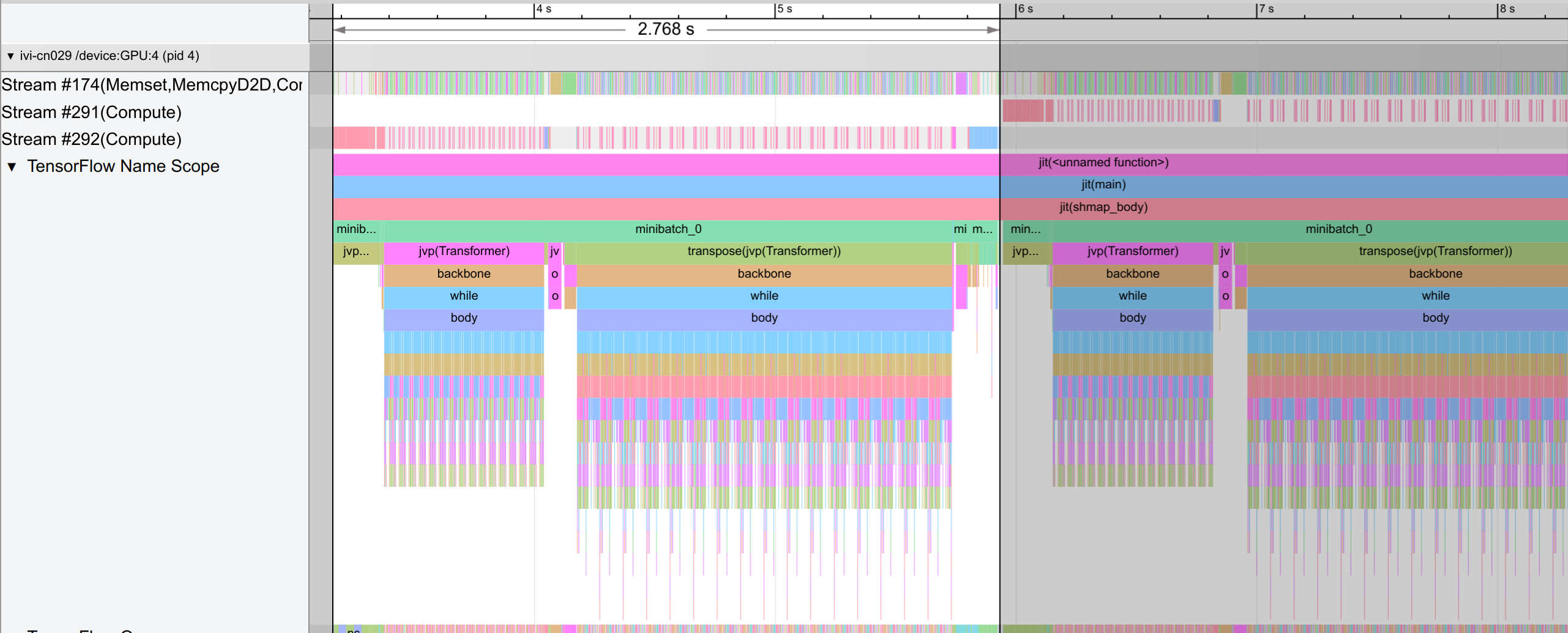
One difference to the single-GPU case is that we have a trace per GPU. In the figure above, we show the trace for GPU-4. A single step takes around 2.8 seconds, and consists of an initial weight gathering across the data axis, the forward pass, and finally the backward pass with remats. Each step in the forward and backward pass iterates over the 16 layers.
Let’s take a closer look at the forward pass below. Specifically, we look at the trace of the MLP block:
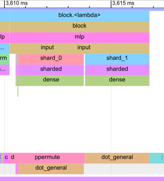
In the input dense layer, we can clearly see how well the communication (ppermute) and computation of shard_0 overlaps. There is only a gap of a few microseconds in which the device is idle.
For the output dense layer, the communication fully overlaps with the computation of the shard_1 output and the dropout. In the trace, the block for ppermute is overlapped with the dot_general operation of shard_1, which makes it a bit more tricky to read.
Now let’s take a look at the attention block below.
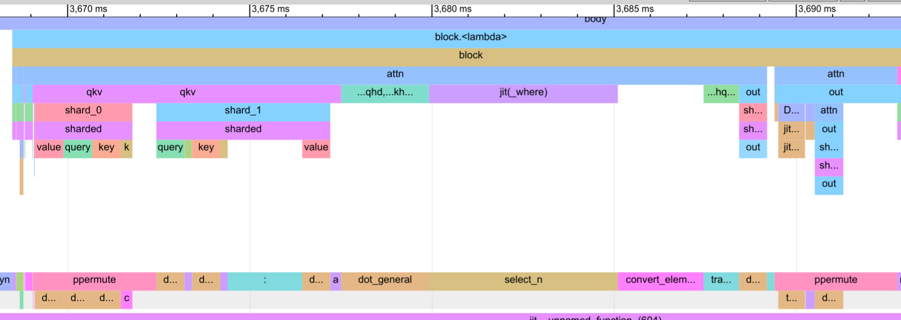
We see that the communication overlap is not as good as for the MLP, and there are some idle gaps in the input and output layer. This is due to the fact that the attention layer has lower computationally complexity in its input and output. For instance, in the input layer, we calculate 3/4-th of the hidden size of the MLP block, and in the output layer, we calculate 1/4-th of the hidden size. This means that the communication would need to be much faster for the attention layer, but our NVLink connections cannot keep up with the speed of the computation (our communication speed in the trace reach close to the 60GB/s limit).
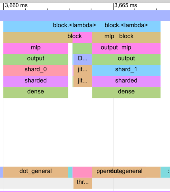
While we could improve it with better communication hardware or larger scale of the model, we can also reduce the communication by parallelizing the attention and the MLP block, as we have done in the parallel block. The trace for the parallel block is shown below.
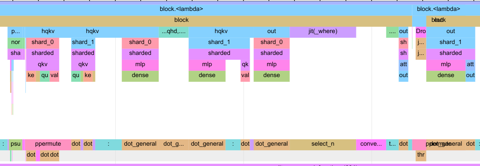
In the input layer, the compiler schedules the query, key and value computations to overlap with the communication. This leads to a small idle gap again in the block, but is overall small compared to the execution time of the block. On the output, however, the communication fully overlaps with the output dense layer of the MLP block. This way, we mitigate the communication gap in the previous version of the attention block, and can reduce the overall execution time of the block. We obtain a step time of 2.6 seconds, which is a 7% improvement over the sequential block.
Still, in our execution, there are a few minor inefficiency in terms of communication, like the gathering and sharding of the model weights over the data axis. We could try to further optimize the model by overlapping communication and computation, and by optimizing the communication pattern. However, we have already reached a very good efficiency with the parallel block, and the remaining inefficiencies are minor compared to the overall execution time. Further, better hardware such as a TPU pod may significantly reduce the inefficiency. In summary, we have successfully profiled a large transformer model with tensor parallelism and fully-sharded data parallelism, and identified potential bottlenecks.
Conclusion
In this notebook, we did a deep-dive into tensor parallelism and how to implement it in JAX. Tensor parallelism is a powerful tool to scale up models to billions of parameters, and is widely used in state-of-the-art models. However, it requires careful consideration of the communication patterns and strategies, and may require adjustments to the model architecture to maximize the efficiency. We started our implementation with parallelizing a simple linear layer over multiple devices, and discussed the communication patterns and strategies to improve the efficiency of the model. In particular, we showed how asynchronous communication can help to overlap communication with compute. We then extended the async gather and scatter strategies to the full transformer model, and discussed the parallelization of the attention and MLP block. We implemented the transformer model with tensor parallelism and fully-sharded data parallelism, and trained it on a simple language modeling task. In the next notebook, we will combine all parallelization strategies we have learned so far to implement a full-scale model with tensor parallelism, pipeline parallelism, and data parallelism.
References and Resources
[Shoeybi et al., 2019] Shoeybi, M., Patwary, M., Puri, R., LeGresley, P., Casper, J. and Catanzaro, B., 2019. Megatron-lm: Training multi-billion parameter language models using model parallelism. arXiv preprint arXiv:1909.08053. Paper link
[Wang and Komatsuzaki, 2021] Wang, B., and Komatsuzaki, A., 2021. Mesh transformer jax. GitHub link
[Xu et al., 2021] Xu, Y., Lee, H., Chen, D., Hechtman, B., Huang, Y., Joshi, R., Krikun, M., Lepikhin, D., Ly, A., Maggioni, M. and Pang, R., 2021. GSPMD: general and scalable parallelization for ML computation graphs. arXiv preprint arXiv:2105.04663. Paper link
[Dehghani et al., 2022] Dehghani, M., Gritsenko, A., Arnab, A., Minderer, M. and Tay, Y., 2022. Scenic: A JAX library for computer vision research and beyond. In Proceedings of the IEEE/CVF Conference on Computer Vision and Pattern Recognition (pp. 21393-21398). Paper link
[Yoo et al., 2022] Yoo, J., Perlin, K., Kamalakara, S.R. and Araújo, J.G., 2022. Scalable training of language models using JAX pjit and TPUv4. arXiv preprint arXiv:2204.06514. Paper link
[Chowdhery et al., 2023] Chowdhery, A., Narang, S., Devlin, J., Bosma, M., Mishra, G., Roberts, A., Barham, P., Chung, H.W., Sutton, C., Gehrmann, S., Schuh, P., et al., 2023. Palm: Scaling language modeling with pathways. Journal of Machine Learning Research, 24(240), pp.1-113. Paper link
[Anil et al., 2023] Anil, R., Dai, A.M., Firat, O., Johnson, M., Lepikhin, D., Passos, A., Shakeri, S., Taropa, E., Bailey, P., Chen, Z. and Chu, E., 2023. Palm 2 technical report. arXiv preprint arXiv:2305.10403. Paper link
[Dehghani et al., 2023] Dehghani, M., Djolonga, J., Mustafa, B., Padlewski, P., Heek, J., Gilmer, J., Steiner, A.P., Caron, M., Geirhos, R., Alabdulmohsin, I., Jenatton, R., et al., 2023. Scaling vision transformers to 22 billion parameters. In International Conference on Machine Learning (pp. 7480-7512). PMLR. Paper link
[McKinney, 2023] McKinney, A., 2023. A Brief Overview of Parallelism Strategies in Deep Learning. Blog post link
[Huggingface, 2024] Huggingface, 2024. Model Parallelism. Documentation link
[Google, 2024] JAX Team Google, 2024. SPMD multi-device parallelism with shard_map. Notebook link
[OpenAI, 2024] OpenAI, 2024. GPT-4. Technical Report
[Google, 2024] Gemini Team Google Deepmind, 2024. Gemini. Technical Report
 If you found this tutorial helpful, consider ⭐-ing our repository.
 For any questions, typos, or bugs that you found, please raise an issue on GitHub.