Part 1.2: Profiling and Scaling Single-GPU Transformer Models

Filled notebook:

Author: Phillip Lippe

In the previous part, we have seen how to implement mixed precision training, gradient accumulation, and gradient checkpointing on a simple MLP model. In this part, we will apply these techniques to a transformer model and see how they can help us to train large models with limited resources. We will also see how to profile the model to identify bottlenecks and optimize the performance. It is recommended to go through Part 1.1 before starting this part, as we will be using the same techniques and concepts. We also assume that you are familiar with the transformer model and its components. If you are not, you can refer to the transformer model paper by Vaswani et al. and our transformer tutorial.

This notebook is designed to run on an accelerator, such as a GPU or TPU. If you are running this notebook on Google Colab, you can enable the GPU runtime. You can do this by clicking on Runtime in the top menu, then Change runtime type, and selecting GPU from the Hardware accelerator dropdown. If the runtime fails, feel free to disable the GPU and run the notebook on the CPU. In that case, we recommend to adjust the configuration of the model to fit the available resources.

Prerequisites

To reduce code duplication between notebooks, we import functions from the previous notebook. For this, we have converted the most important functions into a python script and uploaded it to the same repository. If you run on Google Colab, we need to download the python script before importing the functions. If you the notebook locally, it will be already available.

import os
import urllib.request
from urllib.error import HTTPError

# Github URL where python scripts are stored.
base_url = "https://raw.githubusercontent.com/phlippe/uvadlc_notebooks/master/docs/tutorial_notebooks/scaling/JAX/"
# Files to download.
python_files = ["single_gpu.py", "utils.py"]
# For each file, check whether it already exists. If not, try downloading it.
for file_name in python_files:
    if not os.path.isfile(file_name):
        file_url = base_url + file_name
        print(f"Downloading {file_url}...")
        try:
            urllib.request.urlretrieve(file_url, file_name)
        except HTTPError as e:
            print(
                "Something went wrong. Please try to download the file directly from the GitHub repository, or contact the author with the full output including the following error:\n",
                e,
            )

The file utils.py contains some simple functionalities, such as setting the XLA flags we have seen in the previous tutorial. Let’s do that first.

from utils import install_package, set_XLA_flags_gpu

set_XLA_flags_gpu()

We import our standard libraries below.

import functools
from typing import Any, Dict, Tuple

import flax.linen as nn
import jax
import jax.numpy as jnp
import numpy as np
import optax
from tqdm.auto import tqdm

# Install ml_collections on colab
try:
    from ml_collections import ConfigDict
except ModuleNotFoundError:
    install_package("ml_collections")
    from ml_collections import ConfigDict

# Type aliases
PyTree = Any
Metrics = Dict[str, Tuple[jax.Array, ...]]

Finally, we import the functions and modules from our previous tutorial. If you are not familiar with any of these, check out Part 1.1.

from single_gpu import Batch, TrainState, accumulate_gradients, print_metrics

Building an Optimized Transformer Model

In the following section, we will combine mixed precision, gradient checkpointing and gradient accumulation to train a larger Transformer model on a single GPU.

Model Definition

For passing hyperparameters and configurations to our modules, we will make use of ml-collections’ ConfigDict class (docs). A config dict is a dict-like data structure that supports dot access to its keys, and provides a ‘frozen’ version which is useful for JAX.

We start with implementing the MLP layer in the Transformer model. We support mixed precision from before.

class MLPBlock(nn.Module):
    config: ConfigDict
    train: bool

    @nn.compact
    def __call__(self, x: jax.Array) -> jax.Array:
        input_features = x.shape[-1]
        x = nn.LayerNorm(dtype=self.config.dtype, name="pre_norm")(x)
        x = nn.Dense(
            features=self.config.mlp_expansion * input_features,
            dtype=self.config.dtype,
            name="input_layer",
        )(x)
        x = nn.gelu(x)
        x = nn.Dense(
            features=input_features,
            dtype=self.config.dtype,
            name="output_layer",
        )(x)
        x = nn.Dropout(rate=self.config.dropout_rate, deterministic=not self.train)(x)
        return x

Next, we turn to the attention block. To support mixed precision with numerical stability, we cast the attention weights to float32 before the softmax operation, as discussed before. In cases where we would use float16 precision, the dot product could occasionally go out of range, leading to numerical instability (see e.g. Karras et al., 2023). Thus, we cast the query and key tensors to float32 before the softmax operation, and cast the attention weights back to bfloat16 after the softmax operation. Alternatively, one could also keep the query and key tensors in bfloat16 if we are just short of GPU memory. We implement the adjusted dot product attention below:

def dot_product_attention(
    query: jax.Array,
    key: jax.Array,
    value: jax.Array,
    mask: jax.Array | None,
    softmax_dtype: jnp.dtype = jnp.float32,
):
    """Dot-product attention.

    Follows the setup of https://flax.readthedocs.io/en/latest/api_reference/flax.linen/layers.html#flax.linen.dot_product_attention,
    but supports switch to float32 for numerical stability during softmax.

    Args:
        query: The query array, shape [..., num queries, num heads, hidden size].
        key: The key array, shape [..., num keys, num heads, hidden size].
        value: The value array, shape [..., num keys, num heads, hidden size].
        mask: The boolean mask array (0 for masked values, 1 for non-masked). If None, no masking is applied.
        softmax_dtype: The dtype to use for the softmax and dot-product operation.

    Returns:
        The attention output array, shape [..., num queries, num heads, hidden size].
    """
    num_features = query.shape[-1]
    dtype = query.dtype
    scale = num_features**-0.5
    query = query * scale
    # Switch dtype right before the dot-product for numerical stability.
    query = query.astype(softmax_dtype)
    key = key.astype(softmax_dtype)
    weights = jnp.einsum("...qhd,...khd->...hqk", query, key)
    if mask is not None:
        weights = jnp.where(mask, weights, jnp.finfo(softmax_dtype).min)
    weights = nn.softmax(weights, axis=-1)
    # After softmax, switch back to the original dtype
    weights = weights.astype(dtype)
    new_vals = jnp.einsum("...hqk,...khd->...qhd", weights, value)
    new_vals = new_vals.astype(dtype)
    return new_vals

With that, we can implement the attention block below. We use nn.DenseGeneral to implement the linear projections. Depending on the size of the hidden size, it may be beneficial to split the query, key and value projections into multiple smaller projections, also to give the XLA compiler more flexibility to schedule the computation. For simplicity, we use a single layer projection here, which is commonly more efficient for small model sizes.

class AttentionBlock(nn.Module):
    config: ConfigDict
    mask: jax.Array | None
    train: bool

    @nn.compact
    def __call__(self, x: jax.Array) -> jax.Array:
        input_features = x.shape[-1]
        x = nn.LayerNorm(dtype=self.config.dtype, name="pre_norm")(x)
        qkv = nn.DenseGeneral(
            features=(self.config.num_heads, self.config.head_dim * 3),
            dtype=self.config.dtype,
            name="qkv",
        )(x)
        q, k, v = jnp.split(qkv, 3, axis=-1)
        x = dot_product_attention(q, k, v, mask=self.mask, softmax_dtype=self.config.softmax_dtype)
        x = nn.DenseGeneral(
            features=input_features,
            axis=(-2, -1),
            dtype=self.config.dtype,
            name="output_layer",
        )(x)
        x = nn.Dropout(rate=self.config.dropout_rate, deterministic=not self.train)(x)
        return x

We can now combine the two blocks to implement a full Transformer block. In this block, we want to support gradient checkpointing around the two individual blocks. For this, we consider the config to have a remat key, which contains a sequence of names, indicating the functions/modules to remat. We implement the Transformer block below:

class TransformerBlock(nn.Module):
    config: ConfigDict
    mask: jax.Array | None
    train: bool

    @nn.compact
    def __call__(self, x: jax.Array) -> jax.Array:
        # MLP block
        mlp = MLPBlock
        if "MLP" in self.config.remat:
            mlp = nn.remat(mlp, prevent_cse=False)
        x = x + mlp(config=self.config, train=self.train, name="mlp")(x)
        # Attention block
        attn = AttentionBlock
        if "Attn" in self.config.remat:
            attn = nn.remat(attn, prevent_cse=False)
        x = x + attn(config=self.config, mask=self.mask, train=self.train, name="attn")(x)
        return x

With that, we are ready to implement the full Transformer model. We use the scan transformation to scan over the layers of the model to reduce the compilation time. We implement a text-based GPT-style autoregressive model, which uses an embedding layer to embed the input tokens, and a stack of Transformer blocks to process the tokens. We also add a final dense layer to map the output tokens to the vocabulary size. We implement the model below:

class Transformer(nn.Module):
    config: ConfigDict

    @nn.compact
    def __call__(
        self, x: jax.Array, mask: jax.Array | None = None, train: bool = True
    ) -> jax.Array:
        if mask is None and self.config.causal_mask:
            mask = nn.make_causal_mask(x, dtype=jnp.bool_)
        # Input layer.
        x = nn.Embed(
            num_embeddings=self.config.vocab_size,
            features=self.config.hidden_size,
            dtype=self.config.dtype,
            name="embed",
        )(x)
        pos_emb = self.param(
            "pos_emb",
            nn.initializers.normal(stddev=0.02),
            (self.config.max_seq_len, self.config.hidden_size),
        )
        pos_emb = pos_emb.astype(self.config.dtype)
        x = x + pos_emb[None, : x.shape[1]]
        # Transformer blocks.
        block_fn = functools.partial(TransformerBlock, config=self.config, mask=mask, train=train)
        if "Block" in self.config.remat:
            block_fn = nn.remat(block_fn, prevent_cse=False)
        if self.config.scan_layers:
            block = block_fn(name="block")
            x, _ = nn.scan(
                lambda module, carry, _: (module(carry), None),
                variable_axes={"params": 0},
                split_rngs={"params": True, "dropout": True},
                length=self.config.num_layers,
            )(block, x, ())
        else:
            for l_idx in range(self.config.num_layers):
                x = block_fn(name=f"block_{l_idx}")(x)
        # Output layer.
        x = nn.LayerNorm(dtype=self.config.dtype, name="post_norm")(x)
        x = nn.Dense(
            features=self.config.num_outputs,
            dtype=self.config.dtype,
            name="output_layer",
        )(x)
        x = x.astype(jnp.float32)
        return x

Initialization

With the model set up, we can continue with the initialization. The initialization process is as usual, besides that we create a more detailed config dict below to specify all hyperparameters in the model. By default, we run with bfloat16 precision and remat the MLP and Attention block. The model has 12 layers with a hidden size of 1024. We also create a config for the data, which we will use to create the example batch. We create batches with 64k tokens, which is large for a single GPU, but language models often train with ~1M tokens per batch. Feel free to change the hyperparameters to see how the model behaves with different settings.

data_config = ConfigDict(
    dict(
        batch_size=64,
        seq_len=512,
        vocab_size=2048,
    )
)
model_config = ConfigDict(
    dict(
        hidden_size=1024,
        dropout_rate=0.1,
        mlp_expansion=4,
        num_layers=12,
        head_dim=128,
        causal_mask=True,
        max_seq_len=data_config.seq_len,
        vocab_size=data_config.vocab_size,
        num_outputs=data_config.vocab_size,
        dtype=jnp.bfloat16,
        softmax_dtype=jnp.float32,
        scan_layers=True,
        remat=("MLP", "Attn"),
    )
)
model_config.num_heads = model_config.hidden_size // model_config.head_dim
optimizer_config = ConfigDict(
    dict(
        learning_rate=4e-4,
        num_minibatches=4,
    )
)
config = ConfigDict(
    dict(
        model=model_config,
        optimizer=optimizer_config,
        data=data_config,
        seed=42,
    )
)

We now create the model and initialize the parameters. We set the optimizer to be Adam with a warmup exponential decay schedule, although the optimizer is not really relevant for the simple example at hand.

model = Transformer(config=config.model)
optimizer = optax.adam(
    learning_rate=optax.warmup_exponential_decay_schedule(
        init_value=0,
        peak_value=config.optimizer.learning_rate,
        warmup_steps=10,
        transition_steps=1,
        decay_rate=0.99,
    )
)

We train the model again on a single example batch. Since we perform autoregressive language modeling as the task, the input are the tokens shifted by one, and the target are the original tokens. We also use a causal mask, specified in the config, to prevent the model from attending to future tokens.

tokens = jax.random.randint(
    jax.random.PRNGKey(0),
    (config.data.batch_size, config.data.seq_len),
    1,
    config.data.vocab_size,
)
batch_transformer = Batch(
    inputs=jnp.pad(tokens[:, :-1], ((0, 0), (1, 0)), constant_values=0),
    labels=tokens,
)

Finally, we initialize the parameters of the model, in the same way as before.

model_rng, state_rng = jax.random.split(jax.random.PRNGKey(config.seed))
params = model.init(
    model_rng,
    batch_transformer.inputs[: config.data.batch_size // config.optimizer.num_minibatches],
    train=False,
)["params"]
state = TrainState.create(
    apply_fn=model.apply,
    params=params,
    tx=optimizer,
    rng=state_rng,
)

Let’s check the number of parameters below.

def get_num_params(state: TrainState) -> int:
    return sum(np.prod(x.shape) for x in jax.tree_util.tree_leaves(state.params))


print(f"Number of parameters: {get_num_params(state):_}")

Number of parameters: 155_877_376

With 150M parameters, the model is still relatively small compared to today’s language models, but still challenging to fit on a single GPU. Furthermore, with a batch size of 64k tokens, the memory consumption of the activations is already significant.

Training

We can now train the model with gradient accumulation. We set the number of gradient accumulation steps to 4, which means that we accumulate the gradients over 4 sub-batches. We first define a loss function, which is very similar to the classification loss we have seen before, adjusted to allow for sequences.

def next_token_pred_loss(
    params: PyTree, apply_fn: Any, batch: Batch, rng: jax.Array
) -> Tuple[PyTree, Metrics]:
    """Next token prediction loss function."""
    logits = apply_fn({"params": params}, batch.inputs, train=True, rngs={"dropout": rng})
    loss = optax.softmax_cross_entropy_with_integer_labels(logits, batch.labels)
    correct_pred = jnp.equal(jnp.argmax(logits, axis=-1), batch.labels)
    batch_size = np.prod(batch.labels.shape)
    step_metrics = {"loss": (loss.sum(), batch_size), "accuracy": (correct_pred.sum(), batch_size)}
    loss = loss.mean()
    return loss, step_metrics

We also adjust the train step to use the new loss function. Everything else remains unchanged in the train step.

@functools.partial(
    jax.jit,
    donate_argnames=(
        "state",
        "metrics",
    ),
)
def train_step_transformer(
    state: TrainState,
    metrics: Metrics | None,
    batch: Batch,
) -> Tuple[TrainState, Metrics]:
    """Training step function.

    Executes a full training step with gradient accumulation for the next-token prediction task.

    Args:
        state: Current training state.
        metrics: Current metrics, accumulated from previous training steps.
        batch: Training batch.

    Returns:
        Tuple with updated training state (parameters, optimizer state, etc.) and metrics.
    """
    # Split the random number generator for the current step.
    rng, step_rng = jax.random.split(state.rng)
    # Determine gradients and metrics for the full batch.
    grads, step_metrics = accumulate_gradients(
        state,
        batch,
        step_rng,
        config.optimizer.num_minibatches,
        loss_fn=next_token_pred_loss,
        use_scan=True,
    )
    # Optimizer step.
    new_state = state.apply_gradients(grads=grads, rng=rng)
    # Accumulate metrics across training steps.
    if metrics is None:
        metrics = step_metrics
    else:
        metrics = jax.tree_map(jnp.add, metrics, step_metrics)
    return new_state, metrics

We now determine the metric shapes and initialize the metric PyTree, as we did before.

_, metric_shapes = jax.eval_shape(
    train_step_transformer,
    state,
    None,
    batch_transformer,
)
metrics = jax.tree_map(lambda x: jnp.zeros(x.shape, dtype=x.dtype), metric_shapes)

Now, we can finally train the model. The goal of the training is not to show the model’s performance, but to show the impact of the different techniques on the memory footprint and training speed. Feel free to experiment with different hyperparameters to see how the model behaves with different settings.

for _ in tqdm(range(4)):
    state, metrics = train_step_transformer(state, metrics, batch_transformer)
final_metrics = jax.tree_map(lambda x: jnp.zeros(x.shape, dtype=x.dtype), metric_shapes)
state, final_metrics = train_step_transformer(state, final_metrics, batch_transformer)
print_metrics(final_metrics, "Final metrics - Transformer")

 Final metrics - Transformer
accuracy: 0.000916
loss: 7.776346

Profiling

To gain further insights into the model execution and see the individual operations, we can profile the model (documentation). In JAX, profiling the model creates a trace file which we can view in tools like Chrome’s Trace Viewer or TensorBoard. We can start the profiling via jax.profiler.start_trace, and stop it with jax.profiler.stop_trace. Alternatively, one can use a context manager to start and stop the profiling. For the profiling, we run three training steps to get a good overview of the model execution and reduce the potential impact of the profiler on the model execution. Further, we can annotate operations in the trace via jax.profiler.StepTraceAnnotation or jax.named_scope, to better understand the model execution. Finally, before stopping the trace, we wait for the last train step to finish by blocking the execution until the metrics are ready. We implement the profiling below:

jax.profiler.start_trace("traces/")
for i in range(3):
    with jax.profiler.StepTraceAnnotation("train_step", step_num=i + 1):
        state, metrics = train_step_transformer(state, metrics, batch_transformer)
metrics["loss"][0].block_until_ready()
jax.profiler.stop_trace()

With the trace generated, we can now visualize the model execution in TensorBoard. For this, we switch to the tab Profiler and load the newest trace file. Under trace_viewer@, we can see the individual operations and their execution time. Additionally, we can inspect the used memory in the memory_viewer tab (select jit_train_step_transformer under modules). The cell below is commented out, as it may take a while to start the TensorBoard, but feel free to run it to inspect the trace on your local machine.

# %load_ext tensorboard
# %tensorboard --logdir traces/single_gpu_transformer

Since the trace will be different for different hyperparameters and different hardware configurations, we have uploaded some example runs here. Feel free to download them and investigate the models yourself. All experiments were run on a single A5000 GPU, which has up to 24GB of memory. Below, we go through some example traces to show the impact of the individual techniques on the model execution, and explain how to read the profiler output.

Profiler Overview

The profiler in TensorBoard is a powerful tool to find understand your model execution and find bottlenecks. For a full overview of the profiler, we recommend the official documentation. Here, we give a brief overview of the most important tabs and how to read the profiler output.

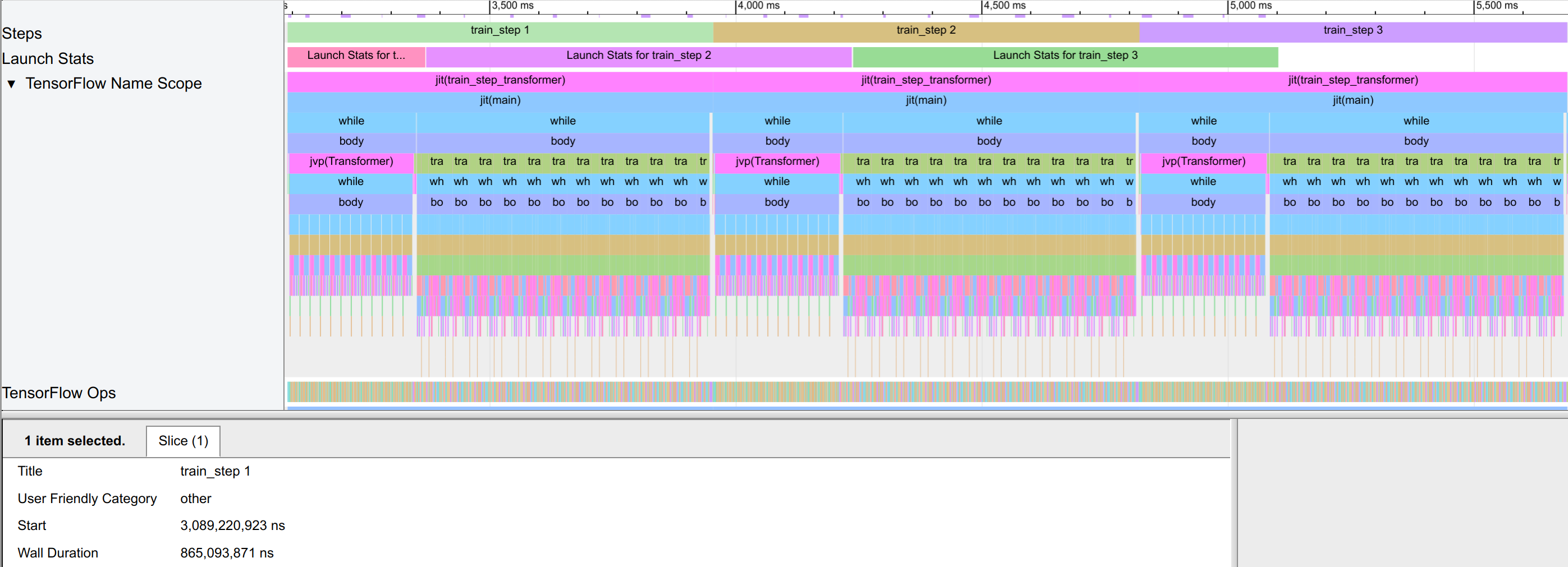
Trace Viewer

The trace viewer is the main tab to inspect the model execution. It shows the individual operations and their execution time. The operations are grouped by the JAX transformation, such as jit, vmap, or scan. We can inspect the execution time of the individual operations, and see which operations take the most time. This can help us to identify potential bottlenecks in the model execution, and optimize the model accordingly. Below is an example view of the trace viewer:

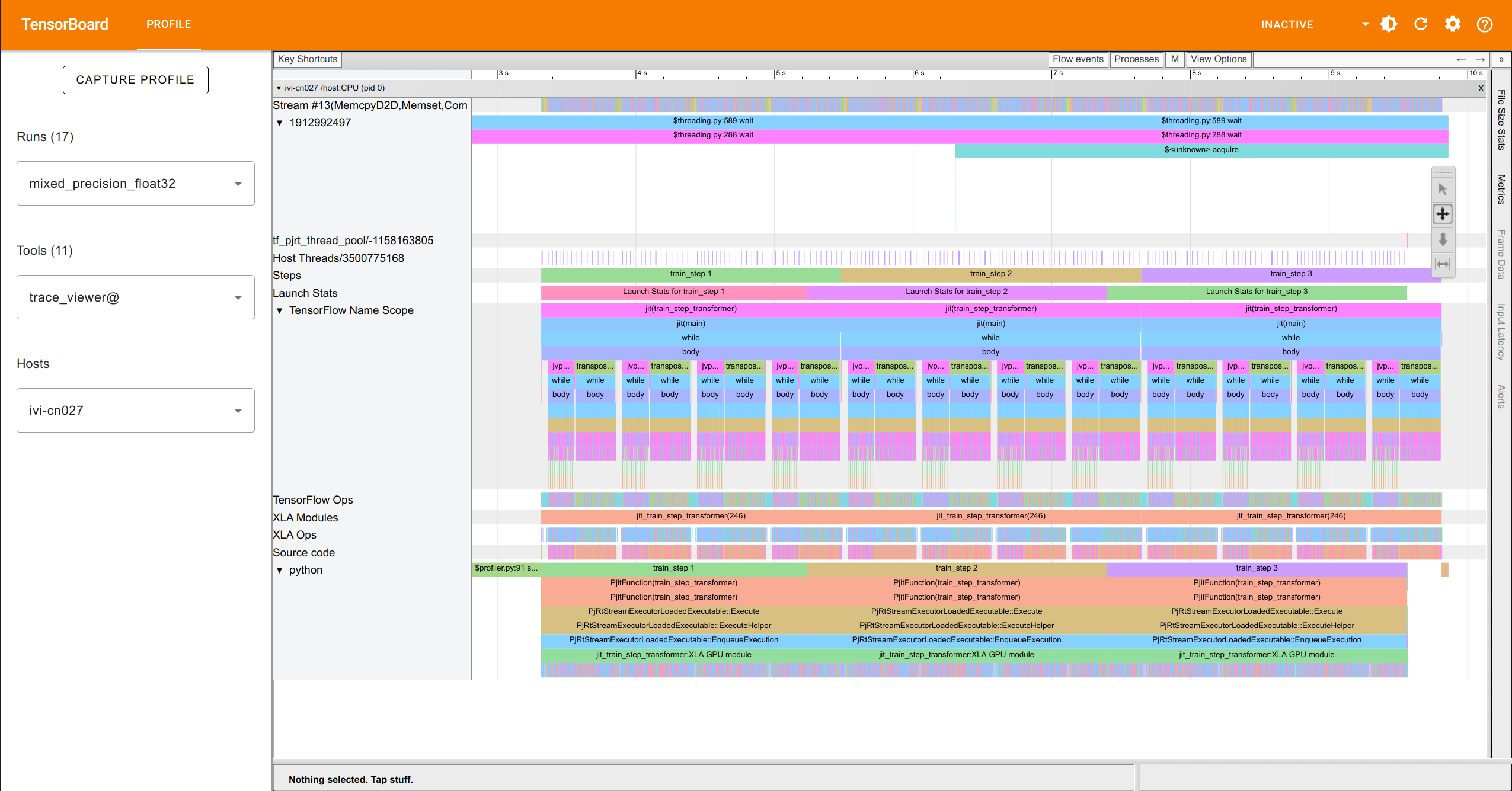
On the left, you have tabs to select the run and hosts if you have multiple nodes. In the middle, you have the individual operations. Here, we are mainly looking at the TensorFlow Name Scope which shows operations with their annotated names (and are most easily understandable for us). On the right, you see the toolbar. The single cursor allows you to select individual blocks and see more details on them (wall clock duration, start time, etc.). The four-way arrow allows you to move around the trace. The up-down arrow allows to zoom into the trace by clicking and dragging up (zoom in) or dragging down (zoom out). This helps us to focus on specific parts of the trace and get down to the individual operations. The left-right arrow allows us to select a subset of the trace and measure the time from one to the other operation. This is helpful for finding the joint execution time of multiple operations together. Overall, in this view, we can see the individual operations and their execution time, and identify potential bottlenecks in the model execution.

Memory Viewer

The memory viewer shows the memory consumption of the model. It shows the memory consumption over operations during the model execution, and how the memory consumption changes over time. This can help us to identify potential memory bottlenecks in the model execution, and optimize the model accordingly. Below is an example view of the memory viewer:

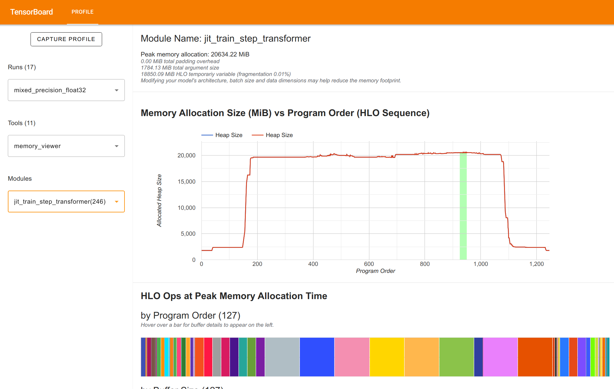
You can hover over the memory graph to find the memory consumption at a specific point in time. Further, on the bottom, you can find the individual arrays that make up the memory consumption. This is very helpful to find the largest memory consumers, and check whether your arrays are all in the right precision and we didn’t forget somewhere to cast them to bfloat16. Overall, in this view, we can see the memory consumption of the model and identify potential memory bottlenecks in the model execution.

We will use both views to understand the impact of the individual techniques on the model execution.

Mixed Precision Training

First, we compare a model in float32 versus bfloat16 precision. For this, we adjust above’s config to remove all remats and set the batch size to 64, to fit in memory. We then profile the model with float32 and bfloat16 precision. In the trace, we look at the memory viewer to get an idea of the memory usage:

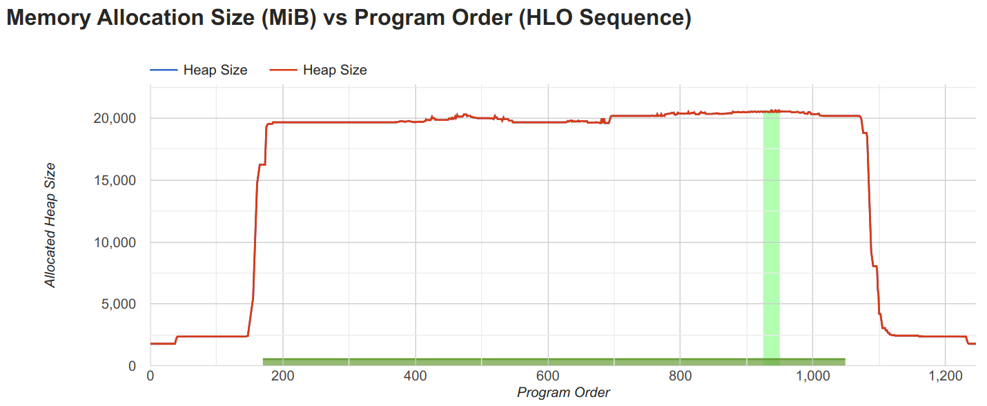
The float32 model is at the maximum of the GPU memory with 20.6GB, while we also already see warnings of JAX that is had to perform automatic rematting. This is a sign that the model is too large to fit into memory. We can further investigate the arrays that take up the most memory in the view below the memory trace.

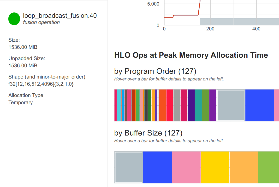
The arrays with largest memory usage are of shape [12, 16, 512, 4096], which are the activations within the MLP block (12 layers, minibatch size 16, 512 sequence length, 4096 hidden size). We can also see that the activations are in float32 precision, which is the main reason for the large memory consumption.

We can now compare this to the bfloat16 model. The memory trace of the bfloat16 model is shown below:

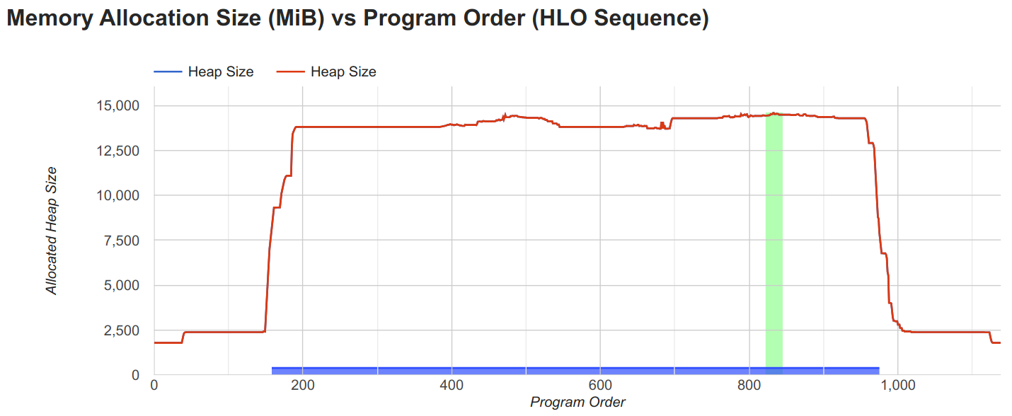
The bfloat16 model is at 14.6GB, which is significantly less than the float32 model. We can also see that the activations are in bfloat16 precision, which is the main reason for the reduced memory consumption. Further, when looking at the largest arrays again, we see that most activations are in bfloat16 precision, and previously largest arrays of shape [12, 16, 512, 4096] are now only half the size in memory (768MB).

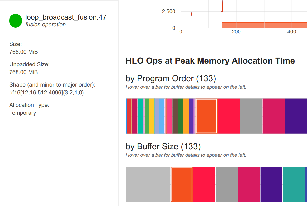
The largest array remaining are the softmax logits in the attention, which with shape [12, 16, 8, 512, 512] are 1.5GB (12 layers, minibatch size 16, 8 attention heads, 512 sequence length). This remains in float32 to prevent numerical instabilities. Overall, this comparison shows the potential of mixed precision training to reduce the memory footprint of the model.

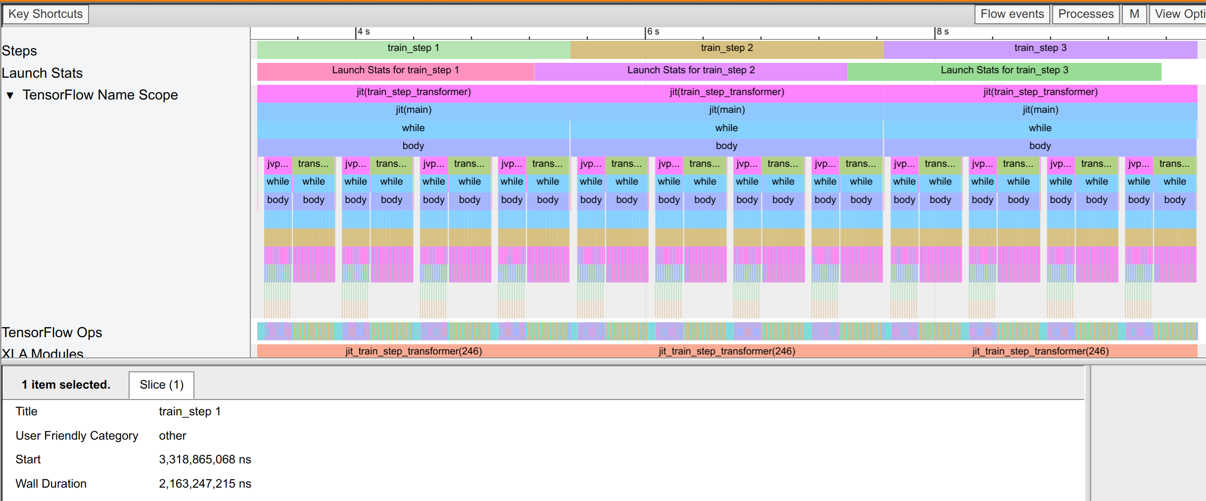
Memory is not the only aspect mixed precision improves. If we look at the trace_viewer tab, we can see that the execution time of the model is also significantly reduced. The float32 precision model takes 2.1 seconds per training step (see wall duration in the picture below). Note that this training step consists of 4 minibatch steps, which we can see in the 4 jvp and transpose blocks per train step.

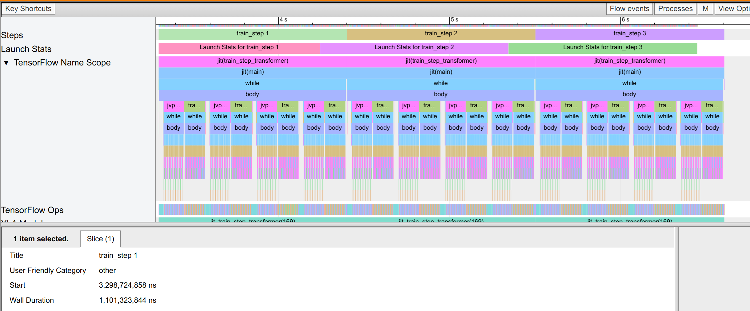
The bfloat16 precision model only takes 1.1 seconds per training step, which is a significant reduction in training time. Each operation can take advantage of the bfloat16 supports of the GPUs tensor cores, which allows for the significant speed up. This shows the potential of mixed precision training to reduce the training time of the model, as well as the memory footprint.

Scanning Layers

Before we continue with the other techniques, we take a closer look at the trace to identify potential model inefficiencies. For this, we zoom in to the trace_viewer tab and look at the individual operations. We see the operation within the block (e.g. mlp and attn), but also that there is quite some gap between the execution of subsequent layers. At closer inspection, many of these gaps are due to the reoccuring operation dynamic_update_slice:

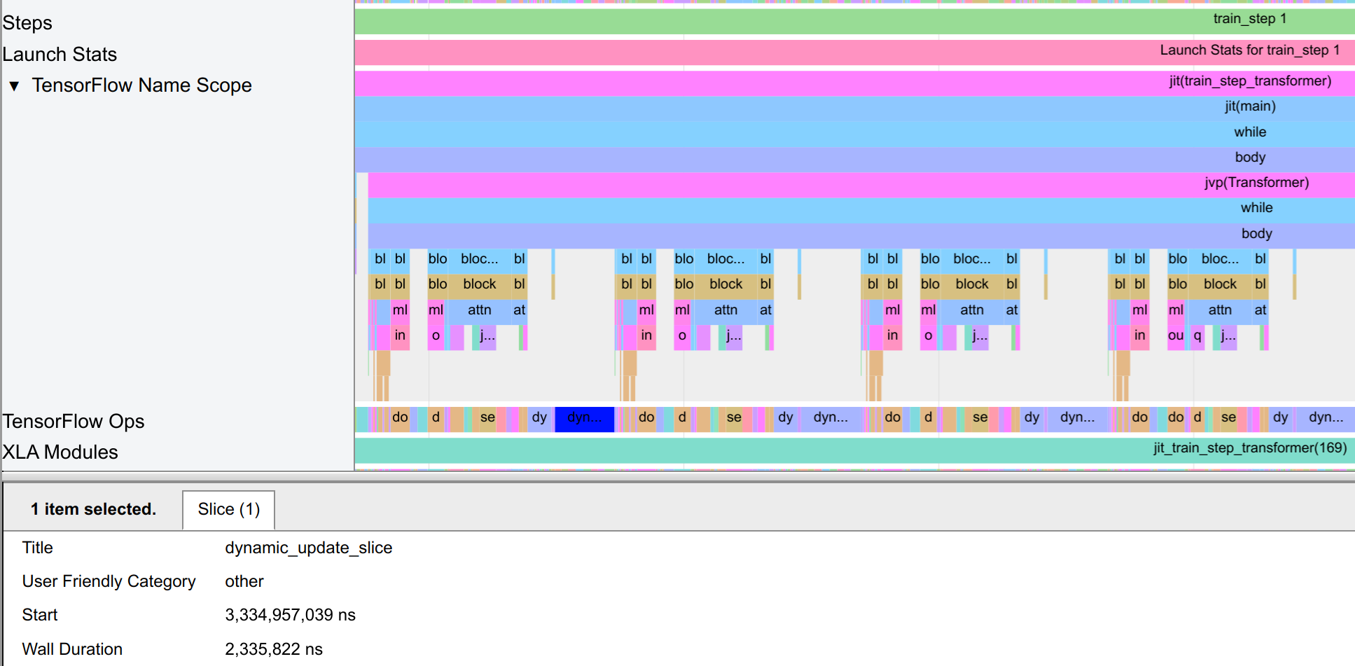
This operation is used to copy one array into another, and is often used in the scan transformation to update the global state of the loop with the buffers of the individual layers. However, we can see that this operation is quite slow since we have to copy large arrays within the GPU memory compared to a fast layer execution. This is a sign that the scan transformation is not optimal for the model, and we should consider sacrificing some compilation time for a more efficient model execution, especially since the model is not extremely deep.

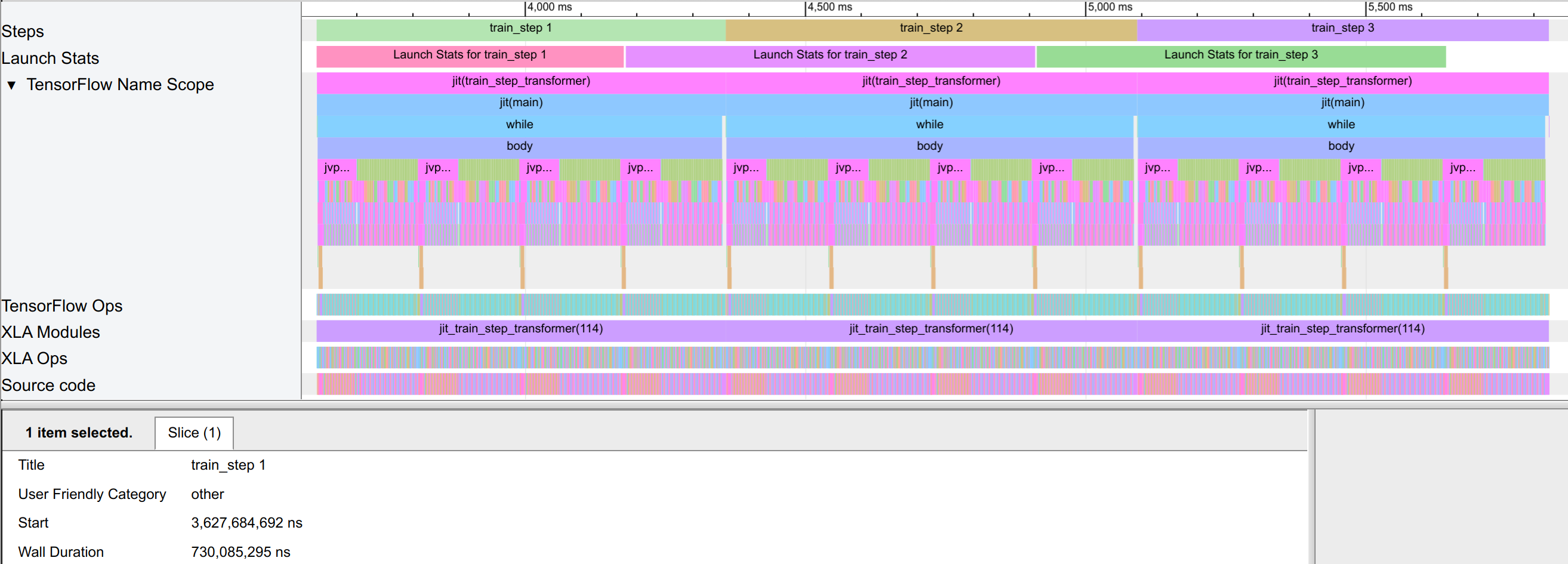
Hence, we test our model with scan_layers=False. While the compilation time increases, it stays within a few seconds, which is negligible for the overall training time. We show the trace of the new model below. We can see that the execution time of the model is significantly reduced to 0.73 seconds instead of 1.1 seconds, and the dynamic_update_slice operations are gone.

Furthermore, the peak memory is also reduced to 8.8GB instead of 14.6GB, which is a significant reduction in memory consumption. This is because we do not enforce the model anymore to keep the full activations of all layers in memory and can release the memory of a layer as soon as the gradients have been calculated:

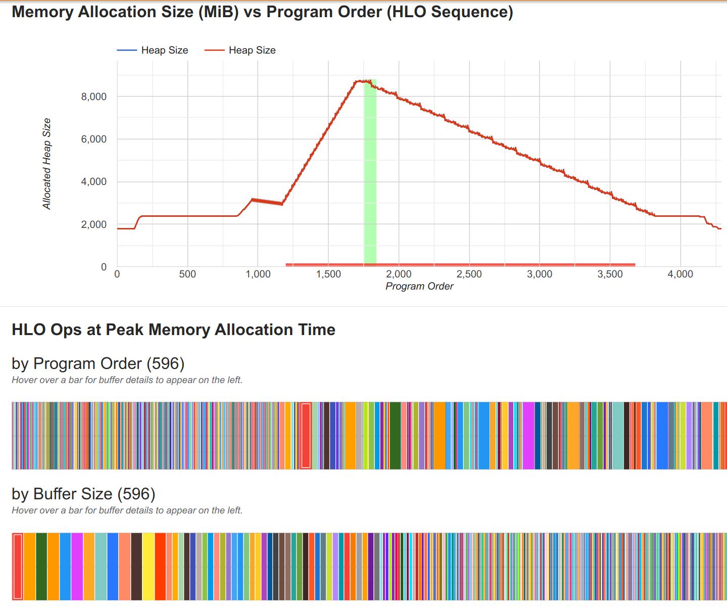
As a result, we find many more small arrays in our buffer, which are the activations of the individual layers. While this can give the compiler more freedom to schedule the computation, we may suffer more from memory fragmentation. However, for the model at hand, this is not a significant issue and we find a significant reduction in memory consumption and execution time when not scanning the layers.

This insight should not be taken as a general rule, but as a reminder to always profile the model and consider the trade-offs of different techniques. For larger models, the scan transformation can be beneficial to reduce the compilation time, but for smaller models, it can be more beneficial to not scan the layers to reduce the memory consumption and execution time.

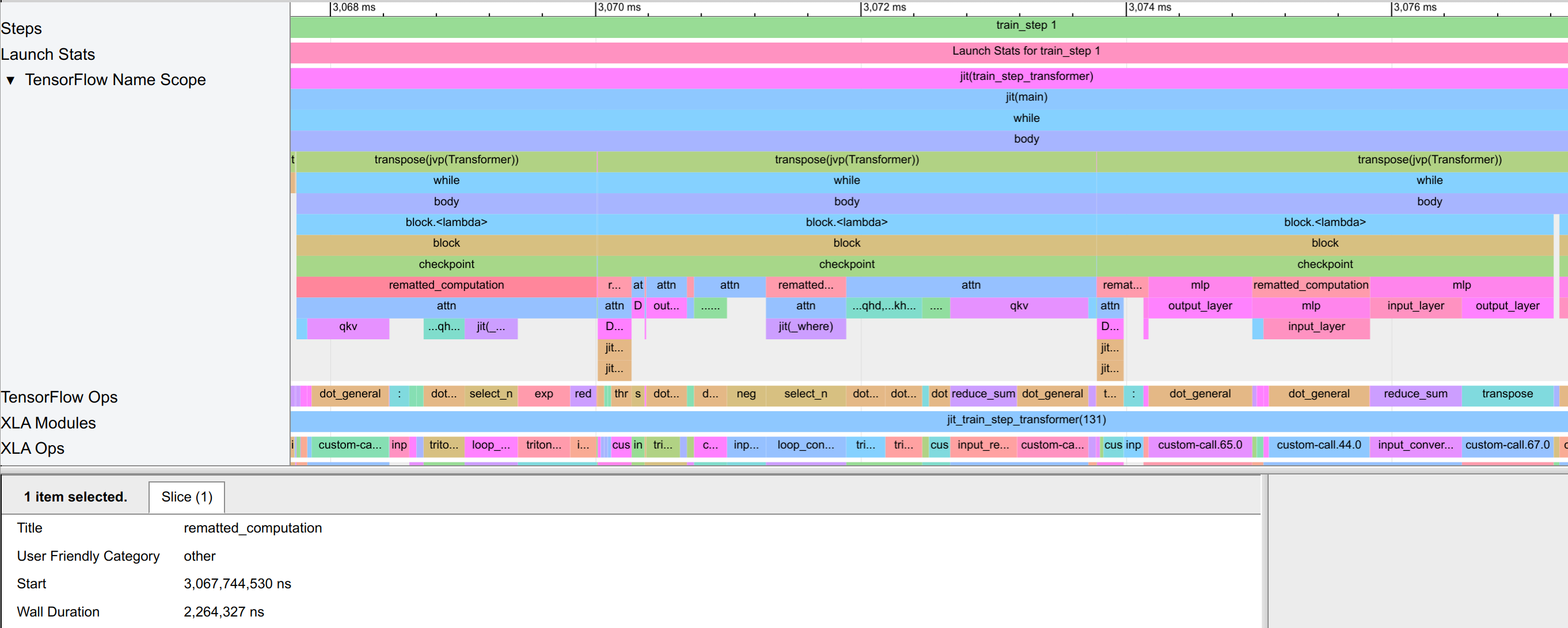
Gradient Checkpointing

Another situation where scanning the layers become efficient again is when we combine it with gradient checkpointing. When recomputing most activations, we reduce the memory that needs to be kept between loop iterations in the scan and thus significantly reduce the dynamic slice operations. For instance, we trace a model using scan and config.remat=("MLP", "Attn"). This corresponds to checkpointing the input activations of the MLP and Attention Block, but recomputing the inner activations of both blocks. We show the trace below:

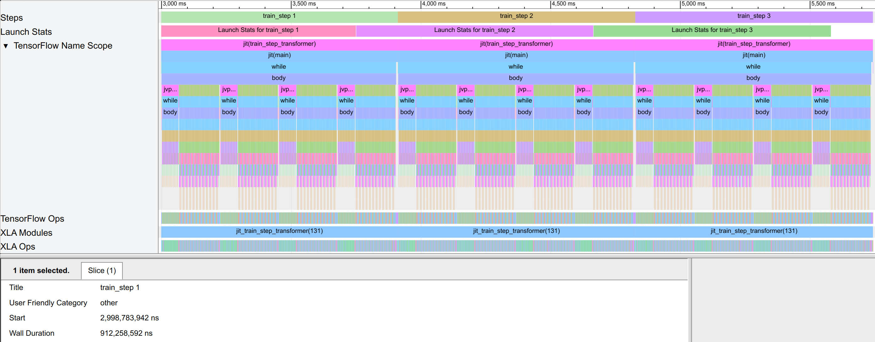
The model takes 0.91 seconds per training step, which is 25% slower than the model without scanning and rematting. Still, the model execution is faster than the scanned model without rematting, since we reduce the memory that needs to be kept between loop iterations. In the trace, the dynamic slice operations take a negligible amount of time now. To also verify that the model is performing the gradient checkpointing as intended, we can zoom into the backward pass of the model. There, we see that in each block, the model is performing rematted_computation blocks, which corresponds to recomputing the activations during the backward pass:

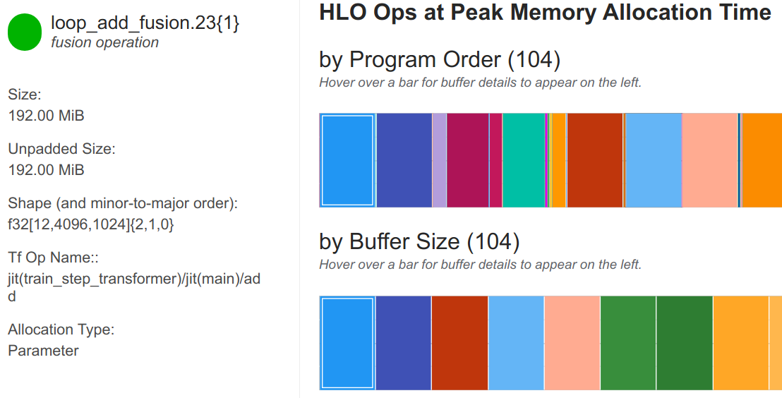
Let’s also check the memory consumption of the model, since this is the main goal of gradient checkpointing. The peak memory, shown below, is reduced to only 3.9GB, which is significantly less than the 14.6GB of the model without rematting.

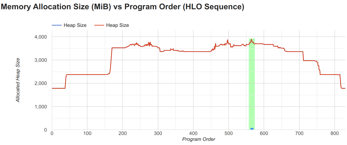
Furthermore, the largest array left in the buffer is the MLP parameters of the model. This indicates that we can significantly increase the model size and batch size with gradient checkpointing, which we could not do with the model without rematting.

Besides rematting the MLP and Attention block, we could also remat the full block. However, since the activations are not the limiting factor for the memory consumption anymore, there is no significant benefit in rematting the full block. We find the model to use 3.8GB of memory, which is only slightly less than the model with rematting the MLP and Attention block. Further, the execution time is also slightly slower with 0.96 seconds per training step, which is likely not worth the small reduction in memory consumption in our case.

Nonetheless, these experiments show the potential of gradient checkpointing to reduce the memory footprint of the model and allow for larger models and batch sizes.

Gradient Accumulation

With mixed precision and gradient checkpointing, we saved so much memory that we do not need gradient accumulation anymore. To check this, we run a model with bfloat16, remat=("MLP","Attn"), and set the number of minibatches to 1, i.e. no gradient accumulation. We first show the memory consumption below:

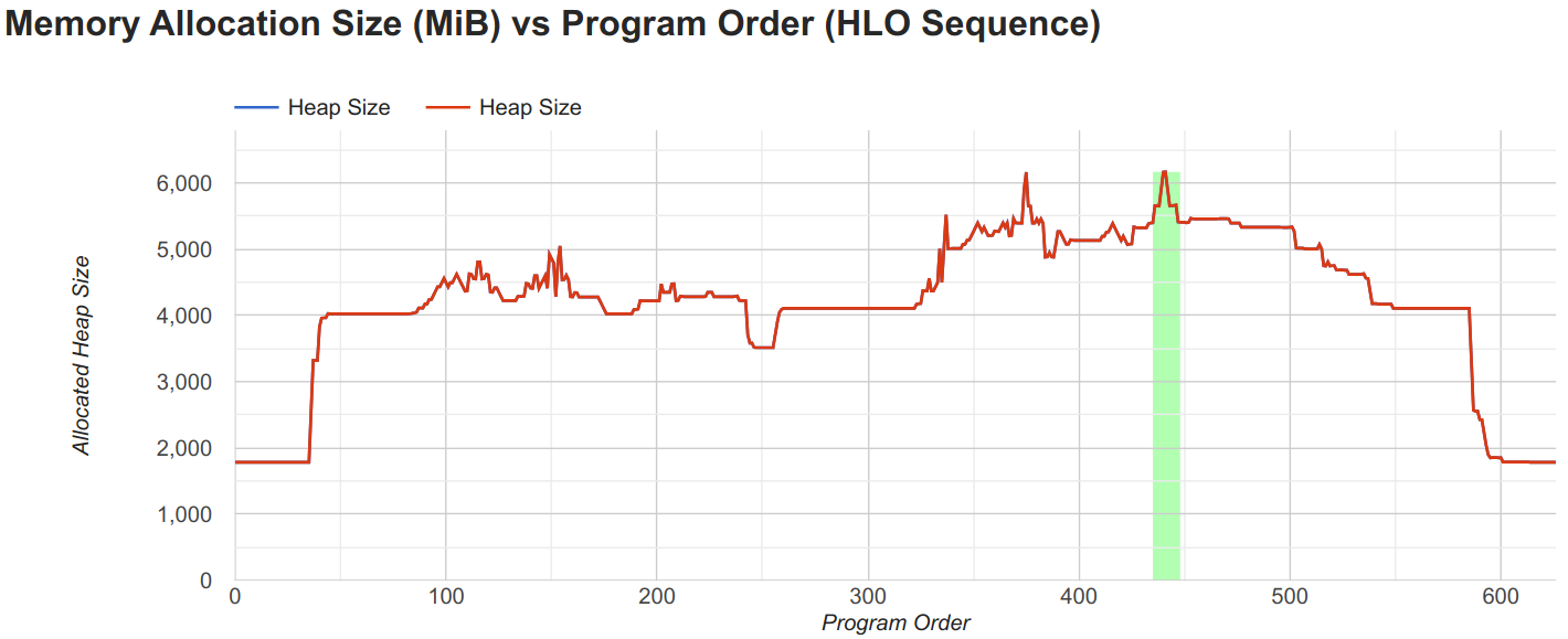
The model takes 6.2GB of memory, which is an increase of the gradient accumulation model, but still significantly less than the maximum GPU memory of 24GB. Further, we can check the execution time of the model by looking at the trace:

With 0.86 seconds per training step, the model is slightly faster than the model with gradient accumulation. This is because the model can parallelize operations better and utilize the GPU more efficiently. Hence, we may want to reduce the usage of gradient accumulation if we have the GPU memory to fit the full batch into it.

Furthermore, we can scale the batch size well beyond 64. For instance, a batch size of 256 fits well into the memory (15GB usage), while the initial model hit the memory limit with a minibatch size of 16. This shows the potential of the combined techniques to reduce the memory footprint of the model and allow for larger models and batch sizes even on a single GPU.

Conclusion

In this notebook, we have explored several techniques to train larger models on a single device. We have implemented mixed precision training, gradient accumulation, and gradient checkpointing on a simple MLP model, and discussed JAX-specific structures to reduce the memory footprint of the model. We have also trained a larger Transformer model with these techniques and profiled the model to gain further insights into the model execution. We have seen that these techniques can significantly reduce the memory footprint of the model and help training larger models. However, these techniques also come with trade-offs, such as increased training time and reduced numerical precision. It is important to carefully consider these trade-offs when training larger models, and to experiment with different techniques to find the best setup for the specific model and hardware configuration. We have also seen that JAX provides a powerful backend with the XLA compiler to optimize our computations on the available hardware, and that we can use the profiler to gain further insights into the model execution. We hope that this notebook has provided a good overview of the techniques to train larger models on a single GPU, and has given a good starting point for further exploration of these techniques. In the following notebooks, we will explore how to train larger models on multiple GPUs and TPUs, and discuss the different parallelization strategies to scale the training to multiple devices.

References and Resources

[Bulatov, 2018] Bulatov, Y., 2018. Fitting larger networks into memory. Blog post link

[Kalamkar et al., 2019] Kalamkar, D., Mudigere, D., Mellempudi, N., Das, D., Banerjee, K., Avancha, S., Vooturi, D.T., Jammalamadaka, N., Huang, J., Yuen, H. and Yang, J., 2019. A study of BFLOAT16 for deep learning training. arXiv preprint arXiv:1905.12322. Paper link

[Ahmed et al., 2022] Ahmed, S., Sarofeen, C., Ruberry, M., et al., 2022. What Every User Should Know About Mixed Precision Training in PyTorch. Tutorial link

[Raschka, 2023] Raschka, S., 2023. Optimizing Memory Usage for Training LLMs and Vision Transformers in PyTorch. Tutorial link (gives more details for the topics here in PyTorch)

[HuggingFace, 2024] HuggingFace, 2024. Performance and Scalability: How To Fit a Bigger Model and Train It Faster. Tutorial link

[NVIDIA, 2024] NVIDIA, 2024. Mixed Precision Training. Documentation link

[NVIDIA, 2024] NVIDIA, 2024. Performance Guide for Training. Documentation link

[Google, 2024] JAX Team Google, 2024. Control autodiff’s saved values with jax.checkpoint (aka jax.remat). Tutorial link

[Google, 2024] JAX Team Google, 2024. Profiling JAX programs. Tutorial link

[Google, 2024] JAX Team Google, 2024. GPU peformance tips. Tutorial link

---

If you found this tutorial helpful, consider ⭐-ing our repository.

For any questions, typos, or bugs that you found, please raise an issue on GitHub.

---