Part 1.1: Training Larger Models on a Single GPU
Filled notebook: 
![]()
Author: Phillip Lippe
When thinking of “scaling” a model, we often think of training a model on multiple GPUs or even multiple machines. However, even on a single GPU, there are many ways to train larger models and make them more efficient. In this notebook, we’ll explore some of these techniques, including mixed precision training, activation checkpointing, gradient accumulation, and more. Most of them aim at reducing the memory footprint of the training step, as memory is commonly the limited resource for single-device training. Moreover, these techniques will be also useful when training on multiple GPUs or TPUs. Hence, it’s important to understand them before diving into distributed training.
We start with discussing each of these techniques separately on a toy example. This will help us understand the impact of each technique on the model’s performance and memory consumption. Then, we’ll combine these techniques to train a larger Transformer model on a single GPU in Part 1.2, and explore the benefits and trade-offs of each technique. Additionally, we will profile the model to get further insights into the efficiency of these techniques.
In this notebook, we will focus on JAX with Flax as the deep learning framework. However, the techniques discussed in this notebook are applicable to other deep learning frameworks like PyTorch as well, and are often implemented in training frameworks like PyTorch Lightning and DeepSpeed. If you are interested in learning more about these techniques in PyTorch, check out the additional resources at the end of this notebook. Further, if you want to closely follow the code in this notebook, it is recommended to have a basic understanding of JAX and Flax. If you are new to JAX and Flax, check out our introduction tutorial to get started.
This notebook is designed to run on CPU or an accelerator, such as a GPU or TPU. If you are running this notebook on Google Colab, you can enable the GPU runtime. You can do this by clicking on Runtime in the top menu, then Change runtime type, and selecting GPU from the Hardware accelerator dropdown. If the runtime fails, feel free to disable the GPU and run the notebook on the CPU.
JAX provides a high-performance backend with the XLA (Accelerated Linear Algebra) compiler to optimize our computations on the available hardware. As JAX continue to be developed, there are more and more features being implemented, that improve efficiency. We can enable some of these new features via XLA flags. At the moment of writing (JAX version 0.4.25, March 2024), the following flags are recommended in the JAX GPU performance tips tutorial and PAX:
[1]:
import os

os.environ["XLA_FLAGS"] = (
    "--xla_gpu_enable_triton_softmax_fusion=true "
    "--xla_gpu_triton_gemm_any=false "
    "--xla_gpu_enable_async_collectives=true "
    "--xla_gpu_enable_latency_hiding_scheduler=true "
    "--xla_gpu_enable_highest_priority_async_stream=true "
)
The last three flags focus on GPU communications, which are not relevant for this notebook, as we are focusing on single-GPU training. For later tutorials, these flags become more relevant.
With the flags set, we can start by importing the necessary libraries and setting up the notebook.
[2]:
import functools
from pprint import pprint
from typing import Any, Callable, Dict, Tuple

import flax.linen as nn
import jax
import jax.numpy as jnp
import numpy as np
import optax
from flax.struct import dataclass
from flax.training import train_state

# Type aliases
PyTree = Any
Metrics = Dict[str, Tuple[jax.Array, ...]]
Mixed Precision Training
As our first technique, we will explore mixed precision training. Mixed precision training is a technique that uses both 16-bit and 32-bit floating-point numbers to speed up training. The idea is to use 16-bit floating-point numbers for most of the computations, as they are faster and require less memory. However, 16-bit floating-point numbers have a smaller range and precision compared to 32-bit floating-point numbers. Therefore, we use 32-bit floating-point numbers for certain computations, such as the model’s weight updates and the final loss computation, to avoid numerical instability.
A potential problem with float16 is that we can encounter underflow and overflow issues during training. This means that the gradients or activations become too large or too small to be represented in the range of float16, and we lose information. Scaling the loss and gradients by a constant factor can help mitigate this issue to bring the values back into the representable range. This is known as loss
scaling, and it is a common technique used in mixed precision training.
As an alternative, JAX and other deep learning frameworks like PyTorch also support the bfloat16 format, which is a 16-bit floating-point format with 8 exponent bits and 7 mantissa bits. The bfloat16 format has a larger range but lower precision compared to the IEEE half-precision type float16, and matches float32 in terms of range. A closer comparison between the formats is
shown in the figure below (figure credit: Google Cloud Documentation):
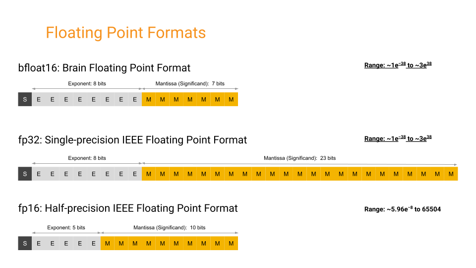
The main benefit of using bfloat16 is that it can be used without loss scaling, as it has a larger range compared to float16. This allows bfloat16 to be used as a drop-in replacement for float32 in many cases to save memory and achieve performances close to float32 (see e.g. JKalamkar et al., 2019). For situations where precision matters over range, float16 may be the better option. Besides memory efficiency, many accelerators like
TPUs and GPUs have native support for bfloat16, which can lead up to 2x speedup in training performance compared to float32 on these devices. Hence, we will use bfloat16 in this notebook.
We implement mixed precision training by lowering all features and activations within the model to bfloat16, while keeping the weights and optimizer states in float32. This is done to keep high precision for the weight updates and optimizer states, while reducing the memory footprint and increasing the training speed by using bfloat16 for the forward and backward passes. While this does not reduce the memory footprint of the model parameters themselves, we often achieve a significant
reduction in memory consumption due to the reduced memory footprint of the activations without influencing the model’s performance. If the model itself is too large to fit into memory, one can also apply lower precision to the model parameters and/or optimizer (e.g. 1-bit Adam), but we will not cover this in this notebook.
Let’s start by implementing mixed precision training on a toy example. We will use a simple MLP model for classification below. In Flax, we can control the data type of most modules in two ways: param_dtype is the data type in which the parameters are stored, and dtype is the data type in which the calculations are performed. We will set param_dtype to float32 and dtype to bfloat16 for the model’s layers and activations. Other layers that do not require parameters, such
as the activation functions or dropout layers, commonly use the data type of the input, which will be bfloat16 in our case. To prevent numerical instabilities, it is commonly recommended to keep large reductions such as in softmax in float32 (see e.g. here). Hence, we cast the final output to float32 before computing the log softmax and the loss. With that, we can implement the
mixed precision in Flax as follows:
[3]:
class MLPClassifier(nn.Module):
    dtype: Any
    hidden_size: int = 256
    num_classes: int = 100
    dropout_rate: float = 0.1

    @nn.compact
    def __call__(self, x: jax.Array, train: bool) -> jax.Array:
        x = nn.Dense(
            features=self.hidden_size,
            dtype=self.dtype,  # Computation in specified dtype, params stay in float32
        )(x)
        x = nn.LayerNorm(dtype=self.dtype)(x)
        x = nn.silu(x)
        x = nn.Dropout(rate=self.dropout_rate, deterministic=not train)(x)
        x = nn.Dense(
            features=self.num_classes,
            dtype=self.dtype,
        )(x)
        x = x.astype(jnp.float32)
        x = nn.log_softmax(x, axis=-1)
        return x
We can investigate dtype usage in the model by using the tabulate function in Flax, listing all the parameters and module input/outputs with their dtype. This can be useful to ensure that the model is using the correct data types. Let’s do this below for the original float32 model:
[4]:
x = jnp.ones((512, 128), dtype=jnp.float32)
rngs = {"params": jax.random.PRNGKey(0), "dropout": jax.random.PRNGKey(1)}
model_float32 = MLPClassifier(dtype=jnp.float32)
model_float32.tabulate(rngs, x, train=True, console_kwargs={"force_jupyter": True})
                                      MLPClassifier Summary
┏━━━━━━━━━━━━━┳━━━━━━━━━━━━━━━┳━━━━━━━━━━━━━━━━━━━━┳━━━━━━━━━━━━━━━━━━┳━━━━━━━━━━━━━━━━━━━━━━━━━━┓
┃ path        ┃ module        ┃ inputs             ┃ outputs          ┃ params                   ┃
┡━━━━━━━━━━━━━╇━━━━━━━━━━━━━━━╇━━━━━━━━━━━━━━━━━━━━╇━━━━━━━━━━━━━━━━━━╇━━━━━━━━━━━━━━━━━━━━━━━━━━┩
│             │ MLPClassifier │ - float32[512,128] │ float32[512,100] │                          │
│             │               │ - train: True      │                  │                          │
├─────────────┼───────────────┼────────────────────┼──────────────────┼──────────────────────────┤
│ Dense_0     │ Dense         │ float32[512,128]   │ float32[512,256] │ bias: float32[256]       │
│             │               │                    │                  │ kernel: float32[128,256] │
│             │               │                    │                  │                          │
│             │               │                    │                  │ 33,024 (132.1 KB)        │
├─────────────┼───────────────┼────────────────────┼──────────────────┼──────────────────────────┤
│ LayerNorm_0 │ LayerNorm     │ float32[512,256]   │ float32[512,256] │ bias: float32[256]       │
│             │               │                    │                  │ scale: float32[256]      │
│             │               │                    │                  │                          │
│             │               │                    │                  │ 512 (2.0 KB)             │
├─────────────┼───────────────┼────────────────────┼──────────────────┼──────────────────────────┤
│ Dropout_0   │ Dropout       │ float32[512,256]   │ float32[512,256] │                          │
├─────────────┼───────────────┼────────────────────┼──────────────────┼──────────────────────────┤
│ Dense_1     │ Dense         │ float32[512,256]   │ float32[512,100] │ bias: float32[100]       │
│             │               │                    │                  │ kernel: float32[256,100] │
│             │               │                    │                  │                          │
│             │               │                    │                  │ 25,700 (102.8 KB)        │
├─────────────┼───────────────┼────────────────────┼──────────────────┼──────────────────────────┤
│             │               │                    │            Total │ 59,236 (236.9 KB)        │
└─────────────┴───────────────┴────────────────────┴──────────────────┴──────────────────────────┘

                               Total Parameters: 59,236 (236.9 KB)
[4]:
'\n\n'
As a comparison, we can now tabulate the same model with the bfloat16 data type:
[5]:
model_bfloat16 = MLPClassifier(dtype=jnp.bfloat16)
model_bfloat16.tabulate(rngs, x, train=True, console_kwargs={"force_jupyter": True})
                                       MLPClassifier Summary
┏━━━━━━━━━━━━━┳━━━━━━━━━━━━━━━┳━━━━━━━━━━━━━━━━━━━━┳━━━━━━━━━━━━━━━━━━━┳━━━━━━━━━━━━━━━━━━━━━━━━━━┓
┃ path        ┃ module        ┃ inputs             ┃ outputs           ┃ params                   ┃
┡━━━━━━━━━━━━━╇━━━━━━━━━━━━━━━╇━━━━━━━━━━━━━━━━━━━━╇━━━━━━━━━━━━━━━━━━━╇━━━━━━━━━━━━━━━━━━━━━━━━━━┩
│             │ MLPClassifier │ - float32[512,128] │ float32[512,100]  │                          │
│             │               │ - train: True      │                   │                          │
├─────────────┼───────────────┼────────────────────┼───────────────────┼──────────────────────────┤
│ Dense_0     │ Dense         │ float32[512,128]   │ bfloat16[512,256] │ bias: float32[256]       │
│             │               │                    │                   │ kernel: float32[128,256] │
│             │               │                    │                   │                          │
│             │               │                    │                   │ 33,024 (132.1 KB)        │
├─────────────┼───────────────┼────────────────────┼───────────────────┼──────────────────────────┤
│ LayerNorm_0 │ LayerNorm     │ bfloat16[512,256]  │ bfloat16[512,256] │ bias: float32[256]       │
│             │               │                    │                   │ scale: float32[256]      │
│             │               │                    │                   │                          │
│             │               │                    │                   │ 512 (2.0 KB)             │
├─────────────┼───────────────┼────────────────────┼───────────────────┼──────────────────────────┤
│ Dropout_0   │ Dropout       │ bfloat16[512,256]  │ bfloat16[512,256] │                          │
├─────────────┼───────────────┼────────────────────┼───────────────────┼──────────────────────────┤
│ Dense_1     │ Dense         │ bfloat16[512,256]  │ bfloat16[512,100] │ bias: float32[100]       │
│             │               │                    │                   │ kernel: float32[256,100] │
│             │               │                    │                   │                          │
│             │               │                    │                   │ 25,700 (102.8 KB)        │
├─────────────┼───────────────┼────────────────────┼───────────────────┼──────────────────────────┤
│             │               │                    │             Total │ 59,236 (236.9 KB)        │
└─────────────┴───────────────┴────────────────────┴───────────────────┴──────────────────────────┘

                                Total Parameters: 59,236 (236.9 KB)
[5]:
'\n\n'
As one can see, the model’s parameters are still stored in float32, while the activations and inputs within the model are now in bfloat16. The initial input to the model is in float32, but the result of the first dense layer is casted down to bfloat16 to enable the mixed precision training. The final output of the model is casted back to float32 before computing the log softmax and the loss. In models like the Transformer, where we have a large activation memory footprint
(batch size \(\times\) sequence length \(\times\) hidden size), this can lead to a significant reduction in memory consumption.
The rest of the training setup (loss function, gradient calculation, etc.) remains unchanged from the typical float32 training. That’s why we do not implement the full training loop here, but we will do so for the full transformer model later in this notebook.
Gradient Checkpointing / Activation Recomputation
Another technique to reduce the memory footprint of the activations is gradient checkpointing (this technique is known under several names, including activation checkpointing, activation recomputation, or rematerialization). Gradient checkpointing is a technique that trades compute for memory by recomputing some activations during the backward pass. The idea is to store only a subset of the activations during the forward pass, and recompute the rest of the activations during the backward pass. This can be useful when the memory consumption of the activations is the limiting factor for the model’s size, and the recomputation of the activations is cheaper than storing them. This is often the case for models with a large memory footprint, such as the Transformer, where the activations can be a significant portion of the memory consumption.
As an example, consider a Transformer with only the MLP blocks (for simplicity). Each MLP block consists of two dense layers with a GELU activation in between, and uses a bfloat16 activation (i.e. 2 bytes per activation). We refer to the batch size with \(B\), sequence length with \(S\), and hidden size \(H\). The memory consumption of the activations in the forward pass is its input \(2BSH\) bytes, the input to the GELU activations \(8BSH\) bytes, the input to the output
layer \(8BSH\) bytes, and the dropout mask with size \(BSH\). This results in a total memory consumption of \(19BSH\) bytes (see Korthikanti et al., 2022 for a detailed computation). With gradient checkpointing, we could choose to only keep the original input tensor of size \(2BSH\) and recompute the rest of the activations during the backward pass. This would reduce the memory consumption of the activations by almost 90%, at the cost of
recomputing the activations during the backward pass. This shows the potential of gradient checkpointing to reduce the memory footprint of the activations. We visualize the idea of gradient checkpointing in the figure below. For simplicity, we do not show the residual connections and layer normalization, but the idea is the same.

In JAX and Flax, we can implement gradient checkpointing using the remat function. The remat function allows us to control which intermediate arrays should be saved on the forward pass, and which are recomputed on the backward pass. As a simple example, consider the following function that computes the GELU activation function manually with its approximation (see e.g. Hendrycks and Gimpel, 2016). Note that in practice, we would use the gelu
function from the flax.nn module which is already optimized, but we use this example to illustrate the concept of gradient checkpointing:
[6]:
def gelu(x: jax.Array) -> jax.Array:
    """GeLU activation function with approximate tanh."""
    # This will be printed once every time the function is executed.
    jax.debug.print("Executing GeLU")
    # See https://arxiv.org/abs/1606.08415 for details.
    x3 = jnp.power(x, 3)
    tanh_input = np.sqrt(2 / np.pi) * (x + 0.044715 * x3)
    return 0.5 * x * (1 + jnp.tanh(tanh_input))
In this function, we instantiate several intermediate tensors, which we may need to store during the backward pass and can be expensive for large tensors. Meanwhile, the computation is relatively cheap, such that we would want to compute these tensors during the backward pass instead of storing them. We can use the remat function to control which tensors are stored and which are recomputed during the backward pass. We can use the remat function as follows:
[7]:
def loss_fn(x: jax.Array, remat: bool) -> jax.Array:
    act_fn = gelu
    if remat:
        act_fn = jax.remat(act_fn)
    return jnp.mean(act_fn(x))
If we now transform this function with a jax.grad call, we will see that JAX is executing the function twice (we see the Executing GeLU print statement twice). This is because JAX is computing the forward pass, then releases all intermediate tensors, and then recomputes them again in the backward pass.
[8]:
x = jax.random.normal(jax.random.PRNGKey(0), (100,))
grad_fn = jax.grad(loss_fn)
_ = grad_fn(x, remat=True)
Executing GeLU
Executing GeLU
If we would run the same function without the remat function, we would only see the Executing GeLU print statement once, as JAX would not need to recompute the intermediate tensors during the backward pass.
[9]:
_ = loss_fn(x, remat=False)
Executing GeLU
This shows that the remat function is controlling which tensors are stored and which are recomputed during the backward pass. We will see in the later Transformer example how we can use it in a neural network layer.
In JAX, the XLA compiler can also automatically apply rematerialization to the forward pass when we jit the function. In that case, we do not need to use the remat function explicitly, as the XLA compiler will automatically apply rematerialization to the forward pass. However, it can still be beneficial to use the remat function in some cases, like in scans (see practical notes on remat) or to
manually control which tensors are stored and which are recomputed.
Gradient Accumulation
A common trade-off in training large models is the batch size. A larger batch size can lead to a more accurate estimate of the gradient, but it also requires more memory. In some cases, the batch size is limited by the memory of the accelerator, and we cannot increase the batch size further. In these cases, we can use gradient accumulation to simulate a larger batch size by accumulating the gradients over multiple sub-batches. Each sub-batch is independently processed, and we perform an optimizer step once all sub-batches have been processed. Gradient accumulation can be useful when the memory consumption of the activations is the limiting factor for the model’s size, but we require a larger batch size for training. However, a disadvantage of gradient accumulation is that each sub-batch is processed independently and sequentially, such that nothing is parallelized and we need to ensure that we can still utilize the accelerator to its full potential with the small batch size. The figure below gives an overview of the gradient accumulation process:

In the figure, we have a batch size of 8, and we accumulate the gradients over 4 sub-batches (we refer to sub-batches as minibatches here). Each sub-batch is of size 2, and we process them one by one. After we obtain the gradients for the first minibatch, we can free up all intermediate arrays of the forward and backward pass, and start processing the next minibatch. Once we have processed all minibatches, we can perform an optimizer step. This allows us to simulate a batch size of 8, while only requiring the memory of a batch size of 2.
In JAX and Flax, we have easy control over the gradient accumulation process, since we explicitly calculate the gradients via jax.grad. Let’s implement this process for our simple classification MLP from the mixed precision training. We first create a train state from Flax, which we extend by an RNG for easier handling of dropout.
[10]:
class TrainState(train_state.TrainState):
    rng: jax.Array
We also create a dataclass to store all elements of a batch. In classification, this is usually the input (e.g. an image) and the target (e.g. a label).
[11]:
@dataclass
class Batch:
    inputs: jax.Array
    labels: jax.Array
We now define a loss function, which is still independent of gradient accumulation. The loss function applies the model and computes the cross-entropy loss. We also return a dictionary with metrics, where the key is the name of the metric, and the value is a tuple of the metric (summed over elements) and the number of elements seen. This allows us to compute the average of the metric later.
[12]:
def classification_loss_fn(
    params: PyTree, apply_fn: Any, batch: Batch, rng: jax.Array
) -> Tuple[PyTree, Metrics]:
    """Classification loss function with cross-entropy."""
    logits = apply_fn({"params": params}, batch.inputs, train=True, rngs={"dropout": rng})
    loss = optax.softmax_cross_entropy_with_integer_labels(logits, batch.labels)
    correct_pred = jnp.equal(jnp.argmax(logits, axis=-1), batch.labels)
    batch_size = batch.inputs.shape[0]
    step_metrics = {"loss": (loss.sum(), batch_size), "accuracy": (correct_pred.sum(), batch_size)}
    loss = loss.mean()
    return loss, step_metrics
With this set up, we can implement the gradient accumulation process. Given a batch, we split it into multiple sub-batches, and execute the gradient function of the loss function for each sub-batch. We then accumulate the gradients and return the accumulated gradients. We also accumulate the metrics, such that we can compute the average of the metrics later. Note that we do not need to explicitly free up the memory of the forward and backward pass, as the XLA compiler will automatically release the memory after the gradient function has been executed. We implement it below with an for-loop over the sub-batches:
[13]:
def accumulate_gradients_loop(
    state: TrainState,
    batch: Batch,
    rng: jax.random.PRNGKey,
    num_minibatches: int,
    loss_fn: Callable,
) -> Tuple[PyTree, Metrics]:
    """Calculate gradients and metrics for a batch using gradient accumulation.

    Args:
        state: Current training state.
        batch: Full training batch.
        rng: Random number generator to use.
        num_minibatches: Number of minibatches to split the batch into. Equal to the number of gradient accumulation steps.
        loss_fn: Loss function to calculate gradients and metrics.

    Returns:
        Tuple with accumulated gradients and metrics over the minibatches.
    """
    batch_size = batch.inputs.shape[0]
    minibatch_size = batch_size // num_minibatches
    rngs = jax.random.split(rng, num_minibatches)
    # Define gradient function for single minibatch.
    grad_fn = jax.value_and_grad(loss_fn, has_aux=True)
    # Prepare loop variables.
    grads = None
    metrics = None
    for minibatch_idx in range(num_minibatches):
        with jax.named_scope(f"minibatch_{minibatch_idx}"):
            # Split the batch into minibatches.
            start = minibatch_idx * minibatch_size
            end = start + minibatch_size
            minibatch = jax.tree_map(lambda x: x[start:end], batch)
            # Calculate gradients and metrics for the minibatch.
            (_, step_metrics), step_grads = grad_fn(
                state.params, state.apply_fn, minibatch, rngs[minibatch_idx]
            )
            # Accumulate gradients and metrics across minibatches.
            if grads is None:
                grads = step_grads
                metrics = step_metrics
            else:
                grads = jax.tree_map(jnp.add, grads, step_grads)
                metrics = jax.tree_map(jnp.add, metrics, step_metrics)
    # Average gradients over minibatches.
    grads = jax.tree_map(lambda g: g / num_minibatches, grads)
    return grads, metrics
A disadvantage of the implementation above is that we need to compile the gradient function for each sub-batch, which can be slow. We can avoid this by using the scan transformation in JAX (docs), which allows us to write a for-loop with a single compilation of the inner step. The scan transformation requires the function to take two inputs: the carry and the input x. The carry is the state that is
passed between the steps, and the x input is the input to the current step. The function returns the new carry and any output that we want to gather per step. In our case, the carry is the accumulated gradients and the accumulated metrics of all previous steps, and the x input is the current minibatch index, with which we select the minibatch and RNG to use. As the new carry, we return the updated accumulated gradients and metrics, and do not require a per-step output. We
implement the gradient accumulation with scan below:
[14]:
def accumulate_gradients_scan(
    state: TrainState,
    batch: Batch,
    rng: jax.random.PRNGKey,
    num_minibatches: int,
    loss_fn: Callable,
) -> Tuple[PyTree, Metrics]:
    """Calculate gradients and metrics for a batch using gradient accumulation.

    In this version, we use `jax.lax.scan` to loop over the minibatches. This is more efficient in terms of compilation time.

    Args:
        state: Current training state.
        batch: Full training batch.
        rng: Random number generator to use.
        num_minibatches: Number of minibatches to split the batch into. Equal to the number of gradient accumulation steps.
        loss_fn: Loss function to calculate gradients and metrics.

    Returns:
        Tuple with accumulated gradients and metrics over the minibatches.
    """
    batch_size = batch.inputs.shape[0]
    minibatch_size = batch_size // num_minibatches
    rngs = jax.random.split(rng, num_minibatches)
    grad_fn = jax.value_and_grad(loss_fn, has_aux=True)

    def _minibatch_step(minibatch_idx: jax.Array | int) -> Tuple[PyTree, Metrics]:
        """Determine gradients and metrics for a single minibatch."""
        minibatch = jax.tree_map(
            lambda x: jax.lax.dynamic_slice_in_dim(  # Slicing with variable index (jax.Array).
                x, start_index=minibatch_idx * minibatch_size, slice_size=minibatch_size, axis=0
            ),
            batch,
        )
        (_, step_metrics), step_grads = grad_fn(
            state.params, state.apply_fn, minibatch, rngs[minibatch_idx]
        )
        return step_grads, step_metrics

    def _scan_step(
        carry: Tuple[PyTree, Metrics], minibatch_idx: jax.Array | int
    ) -> Tuple[Tuple[PyTree, Metrics], None]:
        """Scan step function for looping over minibatches."""
        step_grads, step_metrics = _minibatch_step(minibatch_idx)
        carry = jax.tree_map(jnp.add, carry, (step_grads, step_metrics))
        return carry, None

    # Determine initial shapes for gradients and metrics.
    grads_shapes, metrics_shape = jax.eval_shape(_minibatch_step, 0)
    grads = jax.tree_map(lambda x: jnp.zeros(x.shape, x.dtype), grads_shapes)
    metrics = jax.tree_map(lambda x: jnp.zeros(x.shape, x.dtype), metrics_shape)
    # Loop over minibatches to determine gradients and metrics.
    (grads, metrics), _ = jax.lax.scan(
        _scan_step, init=(grads, metrics), xs=jnp.arange(num_minibatches), length=num_minibatches
    )
    # Average gradients over minibatches.
    grads = jax.tree_map(lambda g: g / num_minibatches, grads)
    return grads, metrics
Especially for very large models, where the compilation time will be significant, the scan transformation can lead to a significant speedup of the compilation. However, for the small model in this example, the speedup may be small. We add a small wrapper below to allow for both versions, although we will mainly use the scan version.
[15]:
def accumulate_gradients(*args, use_scan: bool = False, **kwargs) -> Tuple[PyTree, Metrics]:
    if use_scan:
        return accumulate_gradients_scan(*args, **kwargs)
    else:
        return accumulate_gradients_loop(*args, **kwargs)
After having accumulated the gradients of all batches, we can perform the optimizer step. We implement this in the final training step below:
[16]:
def train_step(
    state: TrainState,
    metrics: Metrics | None,
    batch: Batch,
    num_minibatches: int,
) -> Tuple[TrainState, Metrics]:
    """Training step function.

    Executes a full training step with gradient accumulation.

    Args:
        state: Current training state.
        metrics: Current metrics, accumulated from previous training steps.
        batch: Training batch.
        num_minibatches: Number of minibatches to split the batch into. Equal to the number of gradient accumulation steps.

    Returns:
        Tuple with updated training state (parameters, optimizer state, etc.) and metrics.
    """
    # Split the random number generator for the current step.
    rng, step_rng = jax.random.split(state.rng)
    # Determine gradients and metrics for the full batch.
    grads, step_metrics = accumulate_gradients(
        state, batch, step_rng, num_minibatches, loss_fn=classification_loss_fn, use_scan=True
    )
    # Optimizer step.
    new_state = state.apply_gradients(grads=grads, rng=rng)
    # Accumulate metrics across training steps.
    if metrics is None:
        metrics = step_metrics
    else:
        metrics = jax.tree_map(jnp.add, metrics, step_metrics)
    return new_state, metrics
Let’s now test the implementation for training our small classifier on a single batch. We first define the random number generator keys and hyperparameters, and generate the example batch. Feel free to change the hyperparameters to see how the model behaves with different settings.
[17]:
batch_size = 512
num_inputs = 128
num_classes = 100
rng_seed = 0

rng = jax.random.PRNGKey(rng_seed)
data_input_rng, data_label_rng, model_rng, state_rng = jax.random.split(rng, 4)
batch = Batch(
    inputs=jax.random.normal(data_input_rng, (batch_size, num_inputs)),
    labels=jax.random.randint(data_label_rng, (batch_size,), 0, num_classes),
)
We can now create the model and optimizer, and initialize the parameters as usual. We set the dropout rate to 0 to compare the training with and without gradient accumulation.
[18]:
# Zero dropout for checking later equality between training with and without gradient accumulation.
model = MLPClassifier(dtype=jnp.bfloat16, dropout_rate=0.0)
params = model.init(model_rng, batch.inputs, train=False)["params"]
state = TrainState.create(
    apply_fn=model.apply,
    params=params,
    tx=optax.adam(1e-3),
    rng=state_rng,
)
Before we can train, we need to initialize the metric PyTree which we want to pass to the train step. While we could start with metrics=None, as the train step supports, it would be inefficient since we need to compile twice: once for metrics=None, and once for metrics being a PyTree. We can avoid this by inferring the shape and structure of the metric PyTree via jax.eval_shape, which only evaluates the shapes of the train_step without executing the function or compilation.
Once we have the shape, we can initialize a metric PyTree with zeros and pass it to the train step. We implement this below:
[19]:
_, metric_shapes = jax.eval_shape(
    functools.partial(train_step, num_minibatches=4),
    state,
    None,
    batch,
)
print("Metric shapes:")
pprint(metric_shapes)
Metric shapes:
{'accuracy': (ShapeDtypeStruct(shape=(), dtype=int32),
              ShapeDtypeStruct(shape=(), dtype=int32)),
 'loss': (ShapeDtypeStruct(shape=(), dtype=float32),
          ShapeDtypeStruct(shape=(), dtype=int32))}
We then jit the train step, but define the number of minibatches to be a static argument. This means that for every different value of num_minibatches, we will need to recompile the train step, but keep them in cache for the same value of num_minibatches. This is useful in this case where we want to train the model with different number of gradient accumulation steps and compare the outputs.
[20]:
train_step_jit = jax.jit(
    train_step,
    static_argnames="num_minibatches",
)
We finally write a small training loop to train the model.
[21]:
def train_with_minibatches(
    state: TrainState,
    batch: Batch,
    num_minibatches: int,
    num_train_steps: int,
) -> Tuple[TrainState, Metrics]:
    """Small helper function for training loop."""
    train_metrics = jax.tree_map(lambda x: jnp.zeros(x.shape, dtype=x.dtype), metric_shapes)
    for _ in range(num_train_steps):
        state, train_metrics = train_step_jit(state, train_metrics, batch, num_minibatches)
    return state, train_metrics
We also add a small function to print the metrics nicely.
[22]:
def print_metrics(metrics: Metrics, title: str | None = None) -> None:
    """Prints metrics with an optional title."""
    metrics = jax.device_get(metrics)
    lines = [f"{k}: {v[0] / v[1]:.6f}" for k, v in metrics.items()]
    if title:
        title = f" {title} "
        max_len = max(len(title), max(map(len, lines)))
        lines = [title.center(max_len, "=")] + lines
    print("\n".join(lines))
To validate our gradient accumulation implementation, we can compare the results of the model trained with and without gradient accumulation.
[23]:
state_mini1, metrics_mini1 = train_with_minibatches(
    state, batch, num_minibatches=1, num_train_steps=5
)
state_mini4, metrics_mini4 = train_with_minibatches(
    state, batch, num_minibatches=4, num_train_steps=5
)
print_metrics(metrics_mini1, "Minibatch 1")
print_metrics(metrics_mini4, "Minibatch 4")
== Minibatch 1 ===
accuracy: 0.026953
loss: 4.593200
== Minibatch 4 ===
accuracy: 0.026953
loss: 4.593173
We find that the model trained with gradient accumulation has the same loss and accuracy as the model trained without gradient accumulation. Note that small differences can occur due to using limited precision and we have different reduce operations happening in the two setups. In the gradient accumulation, we add the gradients one by one, while in the single batch, we calculate the gradients at once. However, the differences should be small and not affect the overall performance of the model. Additionally, if we would use dropout, we would expect the models to slightly differ due to the different dropout masks being used in the two setups, but the overall performance should be similar.
We could also compare the memory consumption of the two training processes to see the impact of gradient accumulation on the memory footprint, but due to the small model size, the memory consumption is not significantly different. We will see the impact of gradient accumulation on the memory footprint in the later Transformer example.
JAX-Specific Structures
In JAX, we can also use some JAX-specific structures to reduce the memory footprint of the model and help training larger models. These may not be useful for other frameworks like PyTorch, but good to keep in mind for JAX users. We cover two aspects: donating buffers and scanning.
Donating buffers
In JAX, we follow the idea of functional programming where all functions need to be stateless and pure. This means that we cannot modify the input arguments, and we cannot modify other global variables. This is also true for the model parameters, which are passed as arguments to the training step and returned with updated values. This enforces the device to have memory for at least twice the model parameters and optimizer state. However, as the model grows in size, this can become a significant
limitation. To mitigate this, JAX provides a mechanism to donate buffers, which allows us to reuse the memory of the input arguments for the output arguments. This can be useful when the input and output arguments have the same shape and data type, and we do not need the input arguments after the function has been executed. This is often the case for the model parameters and optimizer state, where we do not need the input arguments after the optimizer step has been executed. We can use the
jax.jit function with the donate_argnums/donate_argnames argument to donate buffers. We can donate buffers for the model parameters and optimizer state, which can reduce the memory footprint of the model and help training larger models. We implement this below for the training step:
[24]:
train_step_donated = jax.jit(
    train_step,
    static_argnames="num_minibatches",
    donate_argnames=(
        "state",
        "metrics",
    ),
)
If we now execute the training step with the donate_argnames argument, JAX will try to reuse the input buffers whenever possible. If the buffers are not usable, for instance because the output has different shapes or data types, JAX will allocate new memory for the output and we will see a warning (see more in here). For large models, we want to make sure that JAX can reuse the model parameter and optimizer state buffers, as
this can significantly reduce the memory footprint of the model.
Scanning layers for faster compilation
In JAX, the compilation time can be a significant bottleneck, especially for large models. In the gradient accumulation section, we already have seen how we can use the scan transformation to reduce the compilation time. However, we can also use the lifted scan transformation from Flax to scan over the layers of the model to reduce the compilation time (docs). This can be useful when we
have a large model with many layers, and we want to reduce the compilation time. We can use the scan transformation to compile the forward and backward pass of the individual layer only once, and reuse it throughout the model execution. This can significantly reduce the compilation time, especially for large models. We can implement this for the Transformer model in the later section.
Intermediate Summary
In this notebook, we have discussed several techniques to train larger models on a single device. We have implemented mixed precision training, gradient accumulation, and gradient checkpointing on a simple MLP model. We have also discussed JAX-specific structures to reduce the memory footprint of the model and help training larger models. In the next part (Part 1.2), we will combine these techniques to train a larger Transformer model on a single GPU, and explore the benefits and trade-offs of each technique. We will also profile the model to get further insights into the efficiency of these techniques.
References and Resources
[Chen et al., 2016] Chen, T., Xu, B., Zhang, C. and Guestrin, C., 2016. Training deep nets with sublinear memory cost. arXiv preprint arXiv:1604.06174. Paper link
[Micikevicius et a., 2018] Micikevicius, P., Narang, S., Alben, J., Diamos, G., Elsen, E., Garcia, D., Ginsburg, B., Houston, M., Kuchaiev, O., Venkatesh, G. and Wu, H., 2018, February. Mixed Precision Training. In International Conference on Learning Representations. Paper link
[Bulatov, 2018] Bulatov, Y., 2018. Fitting larger networks into memory. Blog post link
[Kalamkar et al., 2019] Kalamkar, D., Mudigere, D., Mellempudi, N., Das, D., Banerjee, K., Avancha, S., Vooturi, D.T., Jammalamadaka, N., Huang, J., Yuen, H. and Yang, J., 2019. A study of BFLOAT16 for deep learning training. arXiv preprint arXiv:1905.12322. Paper link
[Ahmed et al., 2022] Ahmed, S., Sarofeen, C., Ruberry, M., et al., 2022. What Every User Should Know About Mixed Precision Training in PyTorch. Tutorial link
[Weng et al., 2022] Weng, L., Brockman, G., 2022. Techniques for training large neural networks. Blog link
[Raschka, 2023] Raschka, S., 2023. Optimizing Memory Usage for Training LLMs and Vision Transformers in PyTorch. Tutorial link (gives more details for the topics here in PyTorch)
[HuggingFace, 2024] HuggingFace, 2024. Performance and Scalability: How To Fit a Bigger Model and Train It Faster. Tutorial link
[NVIDIA, 2024] NVIDIA, 2024. Mixed Precision Training. Documentation link
[NVIDIA, 2024] NVIDIA, 2024. Performance Guide for Training. Documentation link
[Google, 2024] JAX Team Google, 2024. Control autodiff’s saved values with jax.checkpoint (aka jax.remat). Tutorial link
[Google, 2024] JAX Team Google, 2024. Profiling JAX programs. Tutorial link
[Google, 2024] JAX Team Google, 2024. GPU peformance tips. Tutorial link
 If you found this tutorial helpful, consider ⭐-ing our repository.
 For any questions, typos, or bugs that you found, please raise an issue on GitHub.